[Analysis] Database overview
Call to the database - SQL
Ludovic Moisan
2022-06-29
Analysis_Database_overview.RmdDatabase overview
Our database is derived from the recordings collected by the NoiseCapture application from 2017 to 2020, particularly those with a tag which has been manually entered by the user, determining the type of sound heard. The first step in our analysis of this database was to check the repartition, accuracy and relevance of the said tags, whether it be for future work of data prediction or environment’s analysis.
The first study to be carried out within the framework of this analysis is the overview of the temporal distribution of the users’ data. Only the UTC time is retrieved during the measurement by the application, so we need to convert this UTC time into local time based on the geographical area of the measurement in order to perform our analysis. Considering this, only the recordings having a geographical measurement could be taken into account in this study. A loss of about 36% of the data is thus to be taken into account (localization not activated by the user for the time of the recording for example). This subset of our data does include both tagged and untagged tracks.
The views are created on the POSTGRE database by the following SQL scripts : [link]
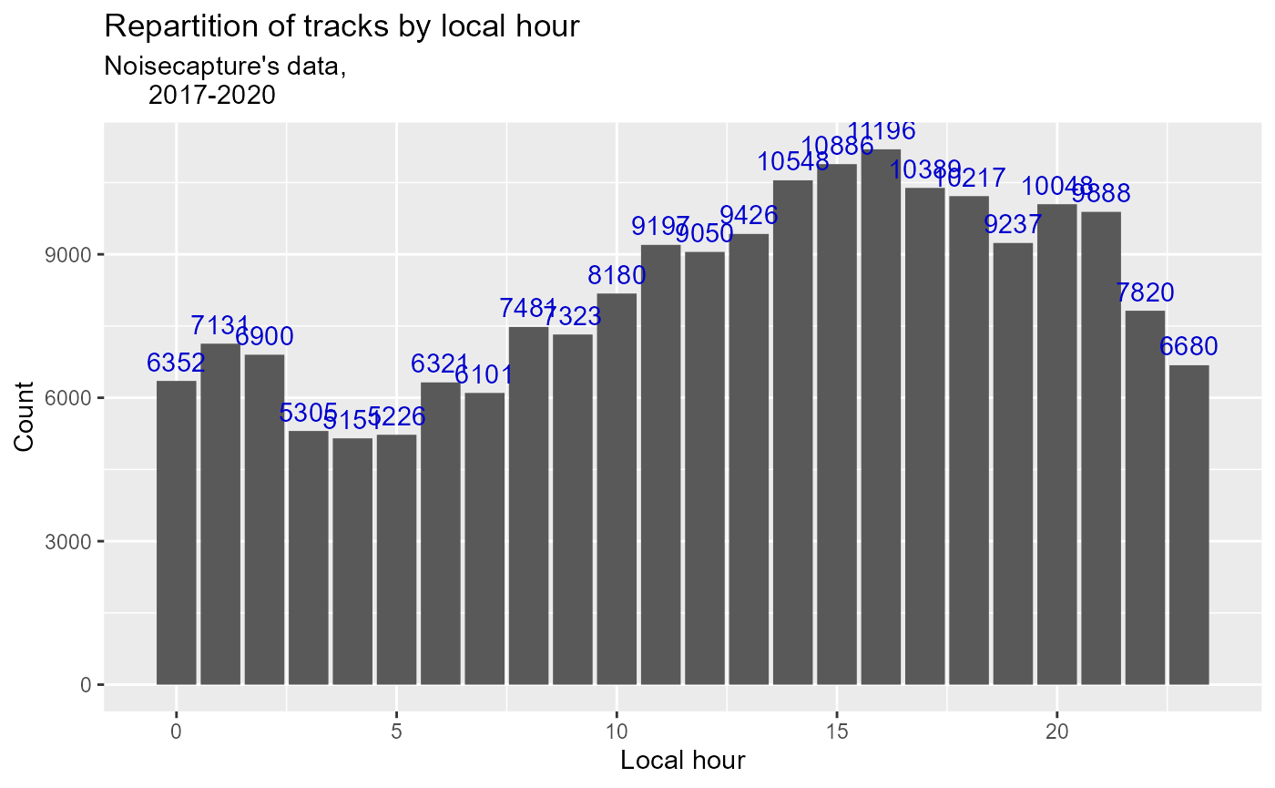
Figure 1: Hourly spread of NoiseCapture usage
The graph above shows us the temporal distribution of the data on a 24h scale. It appears obvious that the use of the application follows the hours of human activity.
As mentioned earlier, the measurements can be divided into two categories, the tracks with tags indicating the nature of the noise recorded (animals, roads etc.) and those without tags. We want to know the distribution of use of this feature.
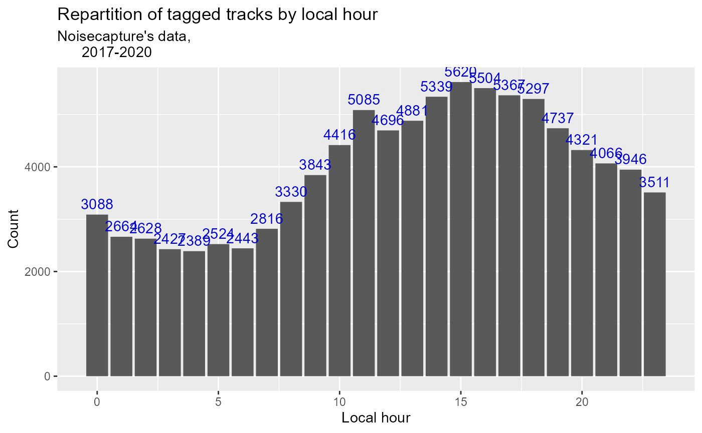
Figure 2: Hourly spread of NoiseCapture tag function usage
The graph above shows us that the dynamics of tag usage is following the global usage of the application previously illustrated.
At first sight, it appeared that our analyses could be biased by the global hourly use when we calculate the percentage of the distribution of the different tags according to the hours of the day. Indeed, the hours of high use could comprise a greater percentage of tagged measurements, or conversely, during hours of low use. In order to verify the limits of interpretation of our data, it is therefore important to verify this hypothesis by calculating the percentage of tagged tracks in relation to the total data over all our hours.
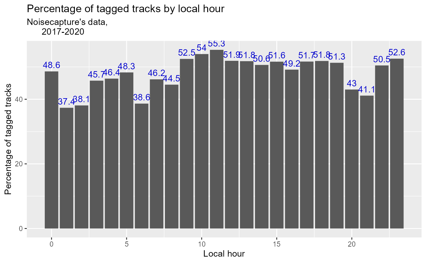
Figure 3: Hourly proportion of NoiseCapture tag function usage
It appears on Figure 3 that the tagged tracks are rather evenly distributed over the hours of the day, with a low standard deviation of 5.19%.
Figure 3 tends to show that the use of tags does not depend much on local time, and can therefore be considered as independent of the global hourly use of the application for our future analyses. In concrete terms, it appears that we can divide the number of tags per hour either by the total number of traces or by the total number of tagged traces, without this making much difference in our visualizations and analyses.