Temporal exploratory analysis

1 Replication

1.1 Get the source code

As the analysis part of project as been treated as R package, there is several ways to get the code source:

using git

git clone https://github.com/nicolas-roelandt/lasso-data-analysis

using R and the remotes package:

# We suggest to use the remotes package
# install.packages("remotes")
remotes::install_github("nicolas-roelandt/lasso-data-analysis")

download as a zip archive

1.2 Setup

This analysis use several packages that you’ll need to install beforehand.

# Package list
pkgs <- c("RPostgreSQL",
          "DBI",
          "sf",
          "dplyr",
          "purrr",
          "ggplot2",
          "scales",
          "lubridate",
          "hydroTSM",
          "suncalc",
          "xfun")

# Packages installation from CRAN
# We suggest to use the remotes package to install required packages
# Already installed packages won't be reinstalled
remotes::install_cran(pkgs)

knitr::opts_chunk$set(echo = TRUE)

# Database connection
library(RPostgreSQL)
library(DBI)
drv <- DBI::dbDriver("PostgreSQL")

# Data handling
library(sf)
library(dplyr)
library(purrr)

# Graphs
library(ggplot2)
library(scales)

# time / date handling
library(lubridate)
library(hydroTSM)

# Get sun rise time
## install.packages("suncalc")
library(suncalc)

# data cache handling
library(xfun)

1.3 Database connection

We provide the database connection parameters to make it easier to replicate and update. However, this database is not publicly available. Those parameters are here to help you connect with your own database (see the README for more information on that aspect.

To help replication, the results of SQL queries have been cached (using the xfun::cache_rds function) and are available as .rds files inside the github repository: https://github.com/nicolas-roelandt/lasso-data-analysis/tree/FOSS4G2022/vignettes/temporal_exploratory_analysis_cache/html

con <- DBI::dbConnect(
drv,
dbname ="noisecapture",
host = "lassopg.ifsttar.fr", #server IP or hostname
port = 5432, #Port on which we ran the proxy
user="noisecapture",
# password stored in .Renviron. To edit : usethis::edit_r_environ()
password=Sys.getenv('noisecapture_password')
)

You can check your connection by requesting the tag list for example.

# Tag list
tag_list <- xfun::cache_rds({
  query <- "SELECT distinct  * FROM noisecapture_tag;"
  RPostgreSQL::dbGetQuery(con,statement = query) 
},rerun = params$database)

tag_list

##    pk_tag       tag_name
## 1      13        natural
## 2      24          noisy
## 3       2          works
## 4       3     mechanical
## 5       8          water
## 6      31          crowd
## 7      16           rail
## 8      36     big street
## 9      18           wind
## 10      4       chatting
## 11      7    air_traffic
## 12     14        animals
## 13     29          birds
## 14     28  heavy vehicle
## 15     33    two-wheeled
## 16     21     vegetation
## 17     22         nature
## 18      1           test
## 19     19           rain
## 20     26  entertainment
## 21      9     industrial
## 22     32       animated
## 23     35   small street
## 24     12           road
## 25     17         alarms
## 26     20 marine_traffic
## 27     11      footsteps
## 28      6         indoor
## 29     30    air-traffic
## 30     25         silent
## 31     15          music
## 32     34        traffic
## 33     27          urban
## 34      5          human
## 35     23      work area
## 36     10       children

2 Data cleaning

The data stored in the database is not useable as is. Most of the data is not taggued, the accuraccy of the GPS position can vary, the track is too long. So the data needs to be filtered.

This has been done within the database using views. Please see the 03_create_views.sql script for more details.

In summary, it removes test and indoor records, filter tracks that have a duration between 5 to 900 seconds. It also remove the tracks where the GPS accuracy was below a 20 meters threshold and that are larger than a 25 square meters area.

This study is focused on France so there is a spatial filtering on its boundaries.

The final data is stored in a view called france_tracks that can be called at will.

2.1 Retrieve data

2.1.1 Track information

track_info <- xfun::cache_rds({
  query <- "SELECT  pk_track, record_utc, time_length, pleasantness, noise_level, track_uuid, geog
FROM france_tracks;"

 sf::st_read(con,query = query)
},rerun = params$database)

track_info %>% head()

## Simple feature collection with 6 features and 6 fields
## Geometry type: GEOMETRY
## Dimension:     XY
## Bounding box:  xmin: -0.5425126 ymin: 45.73464 xmax: 5.000842 ymax: 48.97122
## Geodetic CRS:  WGS 84
##   pk_track          record_utc time_length pleasantness noise_level
## 1     1872 2017-12-14 16:20:17          62           NA       90.54
## 2     1914 2017-09-17 17:51:52          16           75       63.59
## 3     2127 2017-09-05 07:21:26          17          100       59.49
## 4     2236 2018-12-07 14:19:17          13           NA       46.54
## 5     2300 2018-11-11 20:26:18           6           NA       60.88
## 6     2326 2018-11-12 19:04:16          41           NA       72.70
##                             track_uuid                           geog
## 1 f1f6d44c-1399-41fa-8cb9-8becbc43778f POLYGON ((0.6938293 47.3893...
## 2 0acde04f-cb5e-4c4c-bbb4-412f933c3709 POLYGON ((5.000838 45.73464...
## 3 7e508105-e57a-4223-b4b3-ddea7240099f POLYGON ((-0.5425127 47.488...
## 4 8f1bb1ed-814a-4c04-ac01-f7447710766d POLYGON ((4.836361 45.76406...
## 5 18c57c75-05ad-4205-96b5-e5b28580eda1      POINT (2.256505 48.95881)
## 6 947bdf1d-d586-417d-86d9-81a1096cefb9 POLYGON ((2.275491 48.97113...

Some records are not in the France metropolitan area so they need to be discarded.

# Define where to save the dataset
extraWD <- here::here("raw_data")
# Get some data available to anyone
if (!file.exists(file.path(extraWD, "2020_France_metro_WGS84.geojson"))) {
  githubURL <- "https://github.com/nicolas-roelandt/lasso-data-analysis/raw/main/raw_data/2020_France_metro_WGS84.geojson"
  download.file(githubURL, file.path(extraWD, "2020_France_metro_WGS84.geojson"))
  #unzip(file.path(extraWD, "2020_France_metro_WGS84.zip"), exdir = extraWD)
}
france_metro <- sf::st_read(dsn=file.path(extraWD, "2020_France_metro_WGS84.geojson"))

## Reading layer `2020_France_metro_WGS84' from data source 
##   `D:\Roelandt\PROJETS\InProgress\06_UMRAE\2021\lasso-data-analysis\raw_data\2020_France_metro_WGS84.geojson' 
##   using driver `GeoJSON'
## Simple feature collection with 1 feature and 1 field
## Geometry type: MULTIPOLYGON
## Dimension:     XY
## Bounding box:  xmin: -5.141277 ymin: 41.36599 xmax: 9.559961 ymax: 51.08899
## Geodetic CRS:  WGS 84

filtered_track_info <- track_info %>%
  dplyr::filter(sf::st_intersects(., france_metro, sparse = FALSE))

5092 tracks meets the study criteria (duration, envelop area, etc.). 67 tracks where not in France’s metropolitan area.

2.1.2 Tag information

tag_info <- xfun::cache_rds({
  query <- "SELECT ft.pk_track, tag_name FROM france_tracks as ft
INNER JOIN noisecapture_track_tag ntt ON ft.pk_track = ntt.pk_track /* Add track tags*/
INNER JOIN noisecapture_tag ntag ON ntag.pk_tag = ntt.pk_tag /* Add track tags*/;"

 RPostgreSQL::dbGetQuery(con,statement = query) %>% dplyr::filter(pk_track %in% filtered_track_info$pk_track)
})

head(tag_info)

##   pk_track  tag_name
## 1     1872  chatting
## 2     1872  children
## 3     1872 footsteps
## 4     1872     music
## 5     1872      road
## 6     1872      rail

Those 5092 tracks correspond to 9482 tags as a track can have multiple tags.

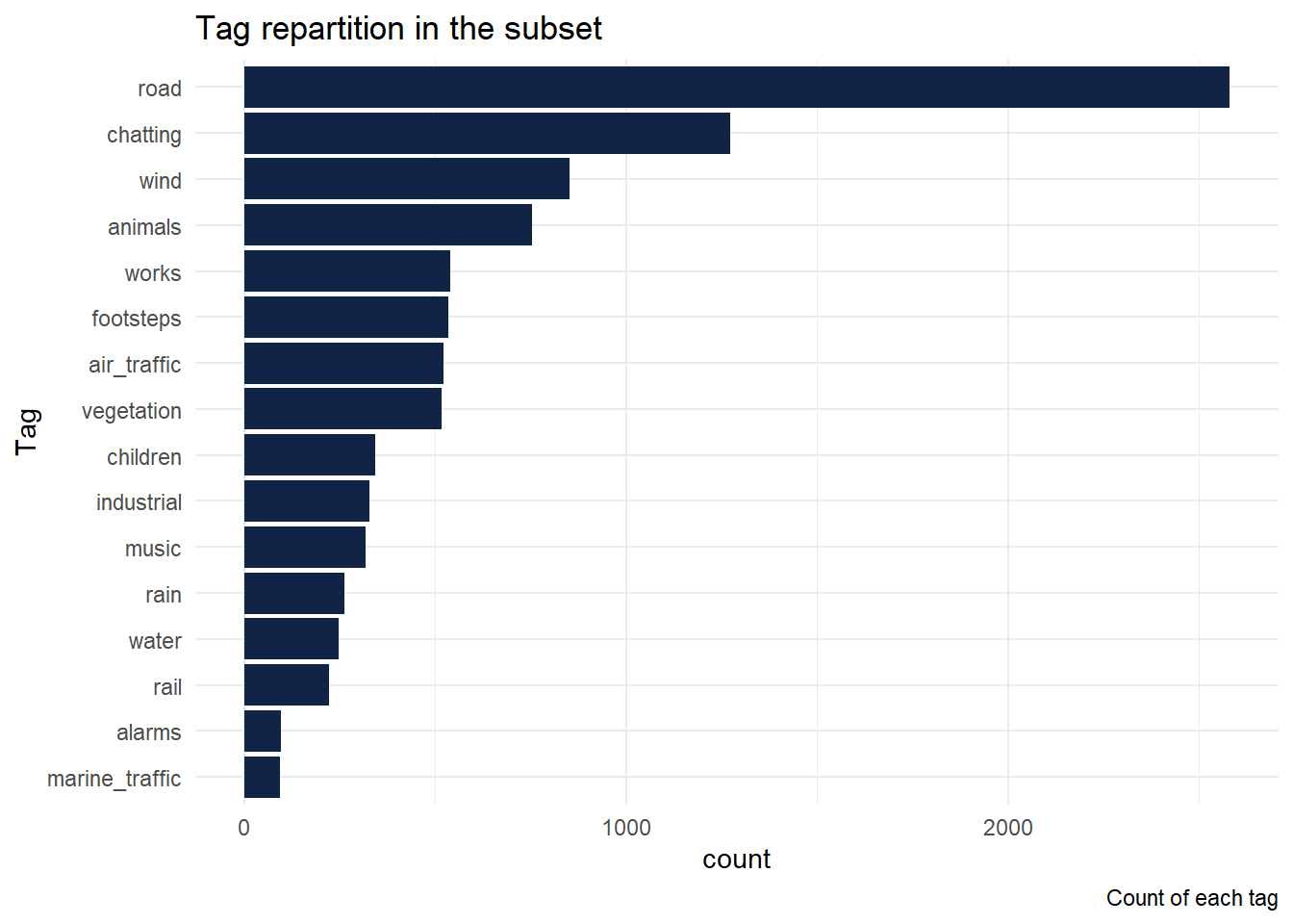
3 Time repartition

3.1 All year

all_info <- tag_info %>% 
  dplyr::inner_join(
    filtered_track_info %>% sf::st_drop_geometry()) %>%
  # add local hour
  dplyr::mutate(local_time = lubridate::hour( # extract hour
    lubridate::with_tz( # convert to local time
      lubridate::ymd_hms(record_utc, tz = "UTC"), # convert text to date
      "Europe/Paris")), # target timezone
    season = hydroTSM::time2season(lubridate::date(record_utc), out.fmt = "seasons", type="default")) # compute season

## Joining, by = "pk_track"

all_info %>% head() %>% knitr::kable()

pk_track	tag_name	record_utc	time_length	pleasantness	noise_level	track_uuid	local_time	season
1872	chatting	2017-12-14 16:20:17	62	NA	90.54	f1f6d44c-1399-41fa-8cb9-8becbc43778f	17	winter
1872	children	2017-12-14 16:20:17	62	NA	90.54	f1f6d44c-1399-41fa-8cb9-8becbc43778f	17	winter
1872	footsteps	2017-12-14 16:20:17	62	NA	90.54	f1f6d44c-1399-41fa-8cb9-8becbc43778f	17	winter
1872	music	2017-12-14 16:20:17	62	NA	90.54	f1f6d44c-1399-41fa-8cb9-8becbc43778f	17	winter
1872	road	2017-12-14 16:20:17	62	NA	90.54	f1f6d44c-1399-41fa-8cb9-8becbc43778f	17	winter
1872	rail	2017-12-14 16:20:17	62	NA	90.54	f1f6d44c-1399-41fa-8cb9-8becbc43778f	17	winter

occurences <- all_info %>% dplyr::group_by(tag_name, local_time) %>% dplyr::count(name = "occurences")

occurences %>% head() %>% knitr::kable()

tag_name	local_time	occurences
air_traffic	0	9
air_traffic	1	1
air_traffic	3	1
air_traffic	4	1
air_traffic	5	1
air_traffic	8	14

tags_hourly_repartition <- occurences %>% 
  left_join(
    occurences %>% dplyr::group_by(local_time) %>% dplyr::summarise(total = sum(occurences)),
    by = "local_time") %>% 
  mutate(percentage = occurences * 100 / total)

tags_hourly_repartition %>% head() %>% knitr::kable()

tag_name	local_time	occurences	total	percentage
air_traffic	0	9	171	5.2631579
air_traffic	1	1	119	0.8403361
air_traffic	3	1	50	2.0000000
air_traffic	4	1	22	4.5454545
air_traffic	5	1	31	3.2258065
air_traffic	8	14	116	12.0689655

ggplot(tags_hourly_repartition) +
  aes(x = local_time, y = percentage) +
  geom_point(shape = "circle", size = 1.5, colour = "#112446") +
  labs(
    x = "Time of the day",
    y = "Percentage",
    title = "Hourly repartition of tags",
    subtitle = "Noicecaptures tags in metropolitan France,
    2017 - 2020"
  ) +
  theme_minimal() +
  facet_wrap(vars(tag_name))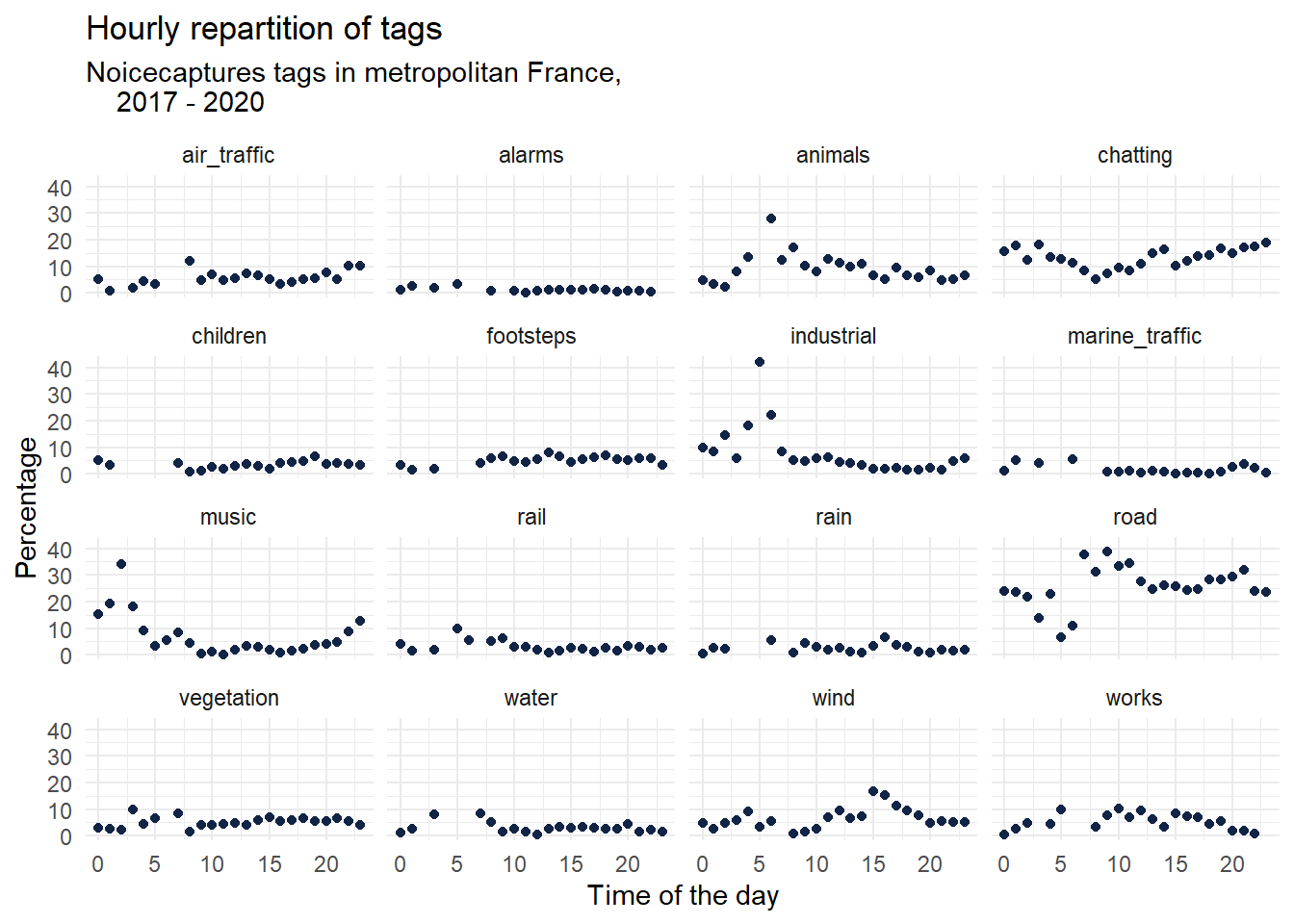

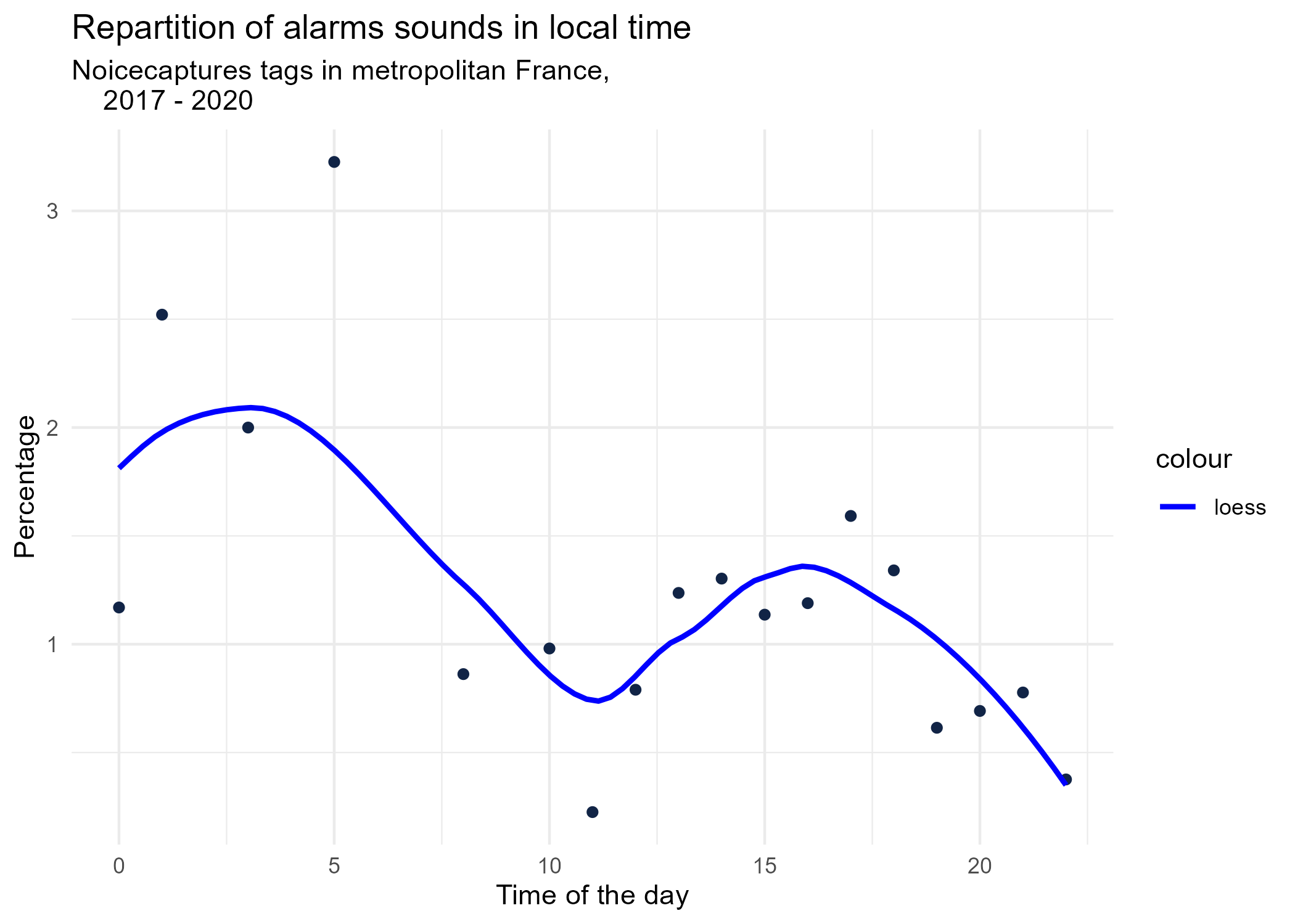
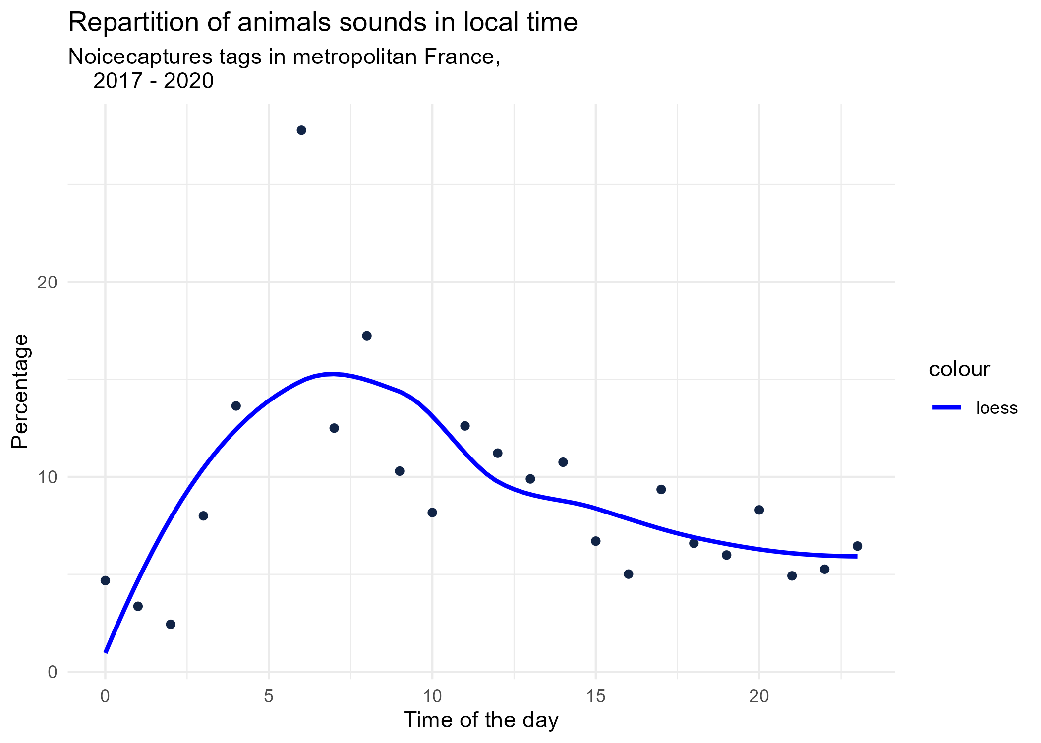
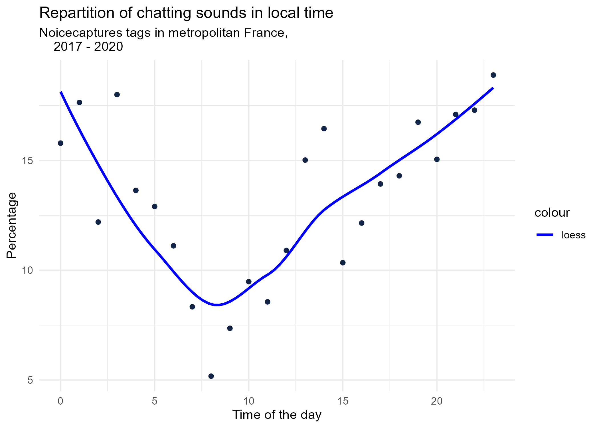
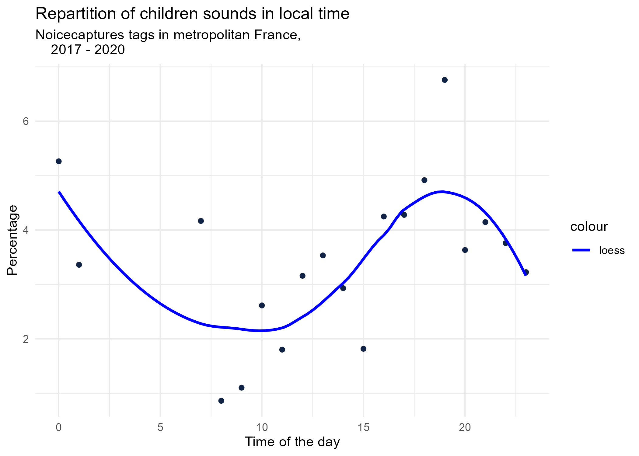
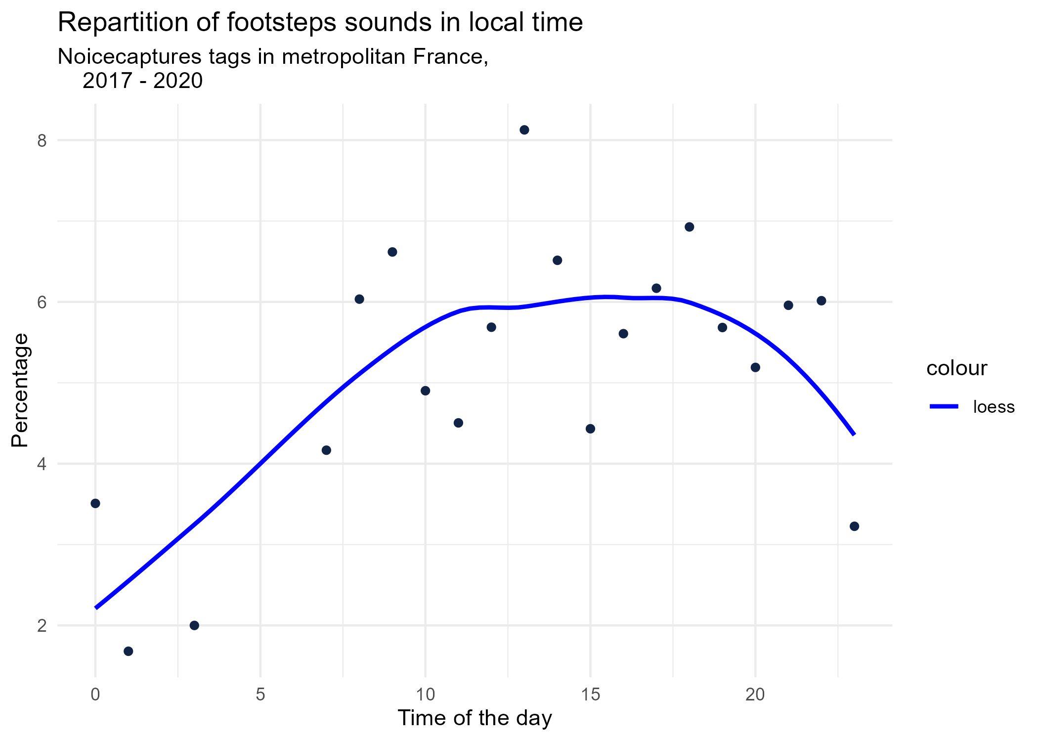
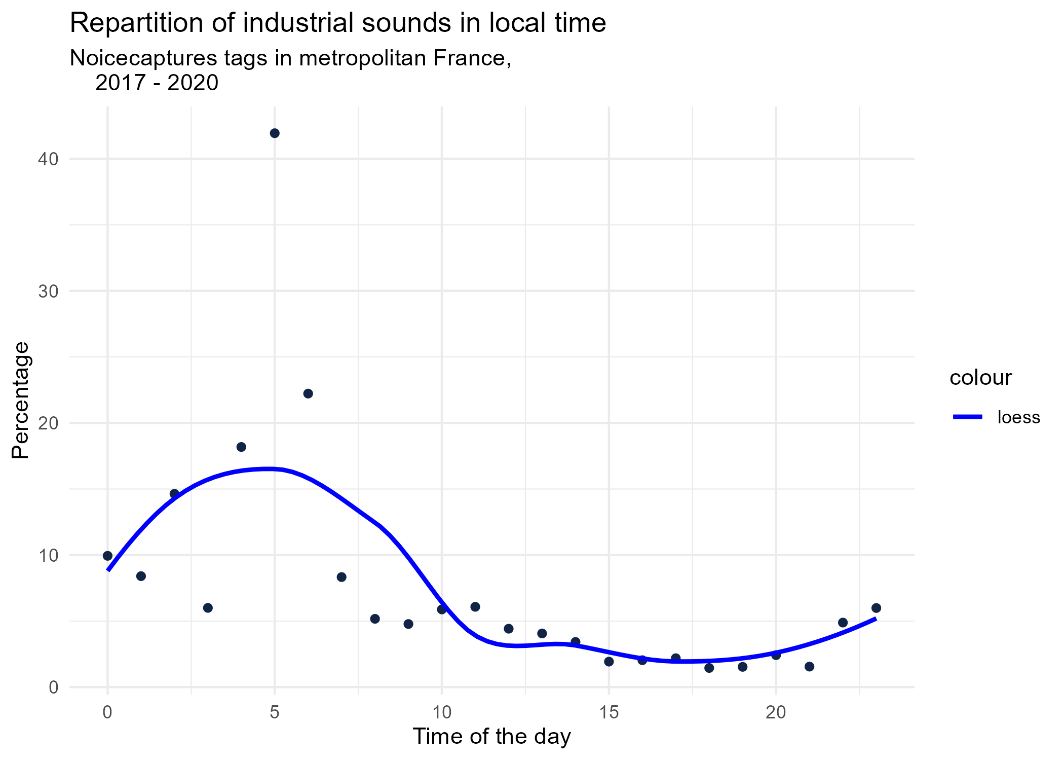
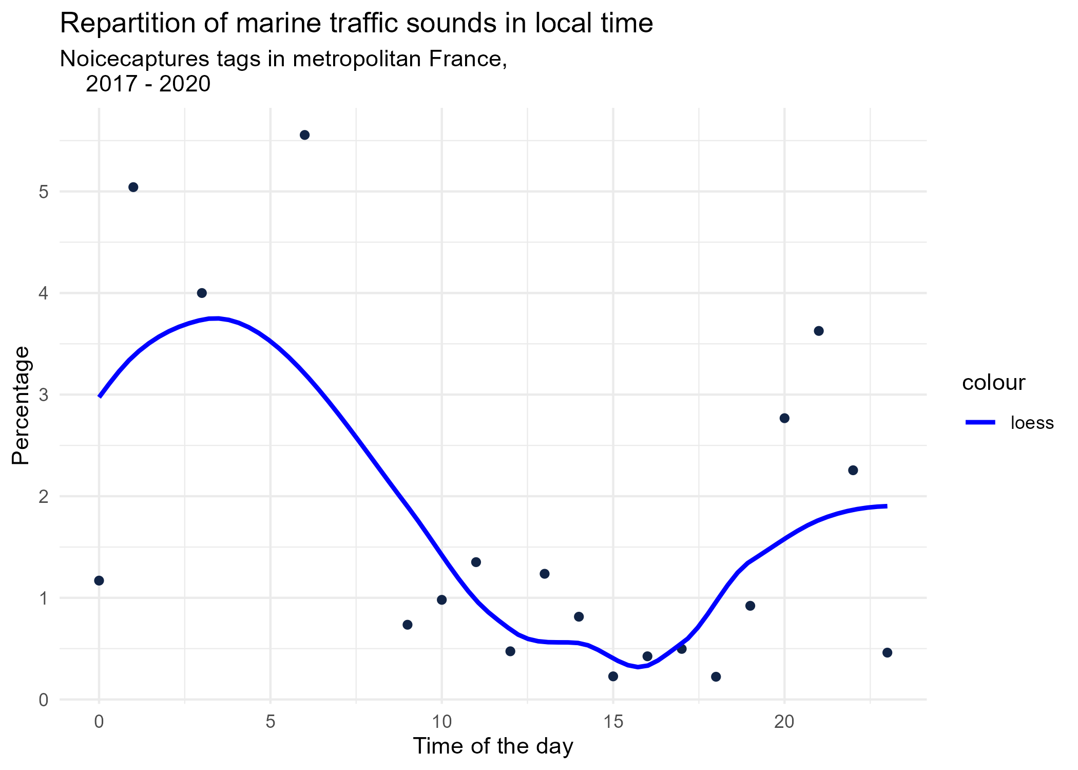
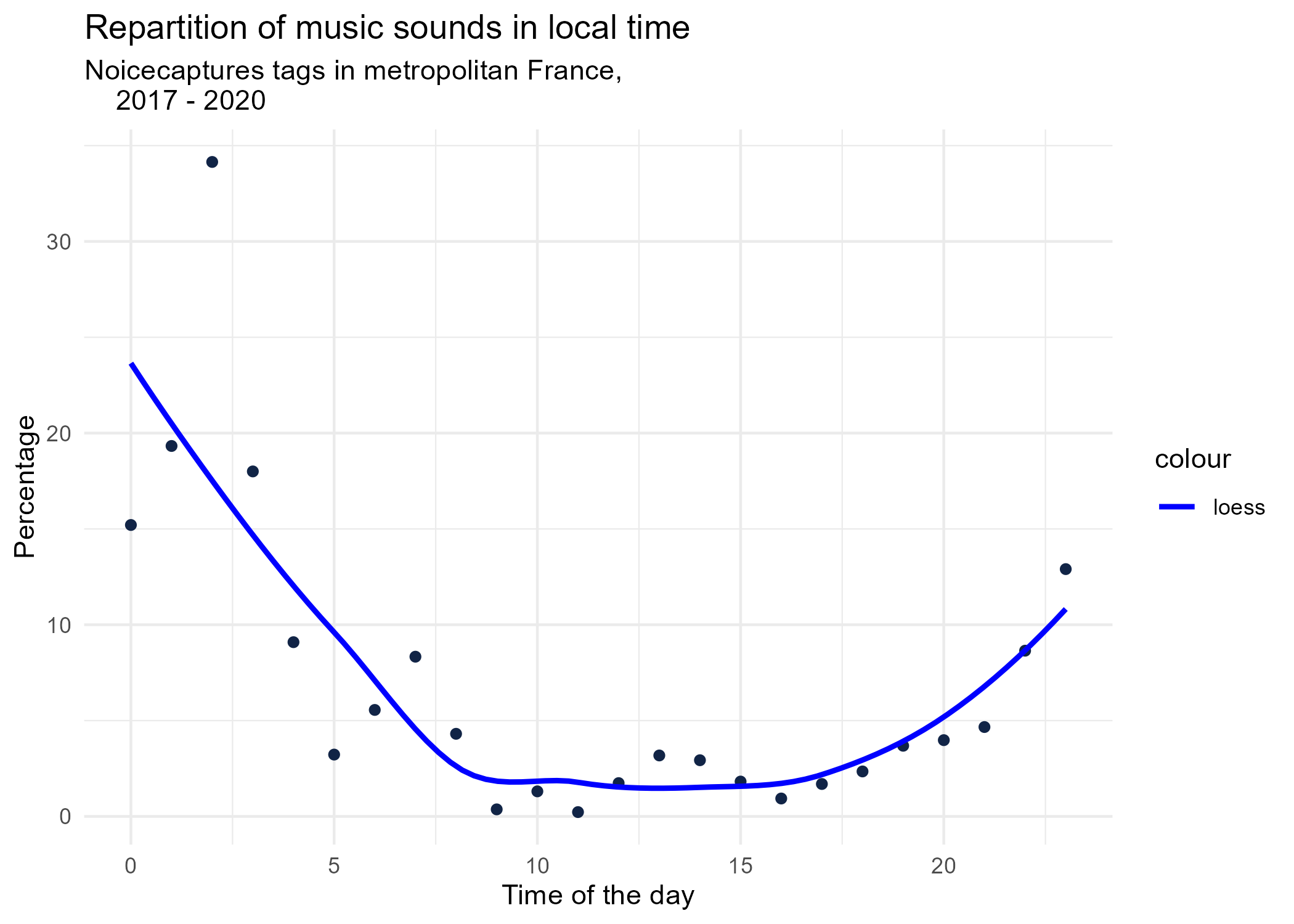
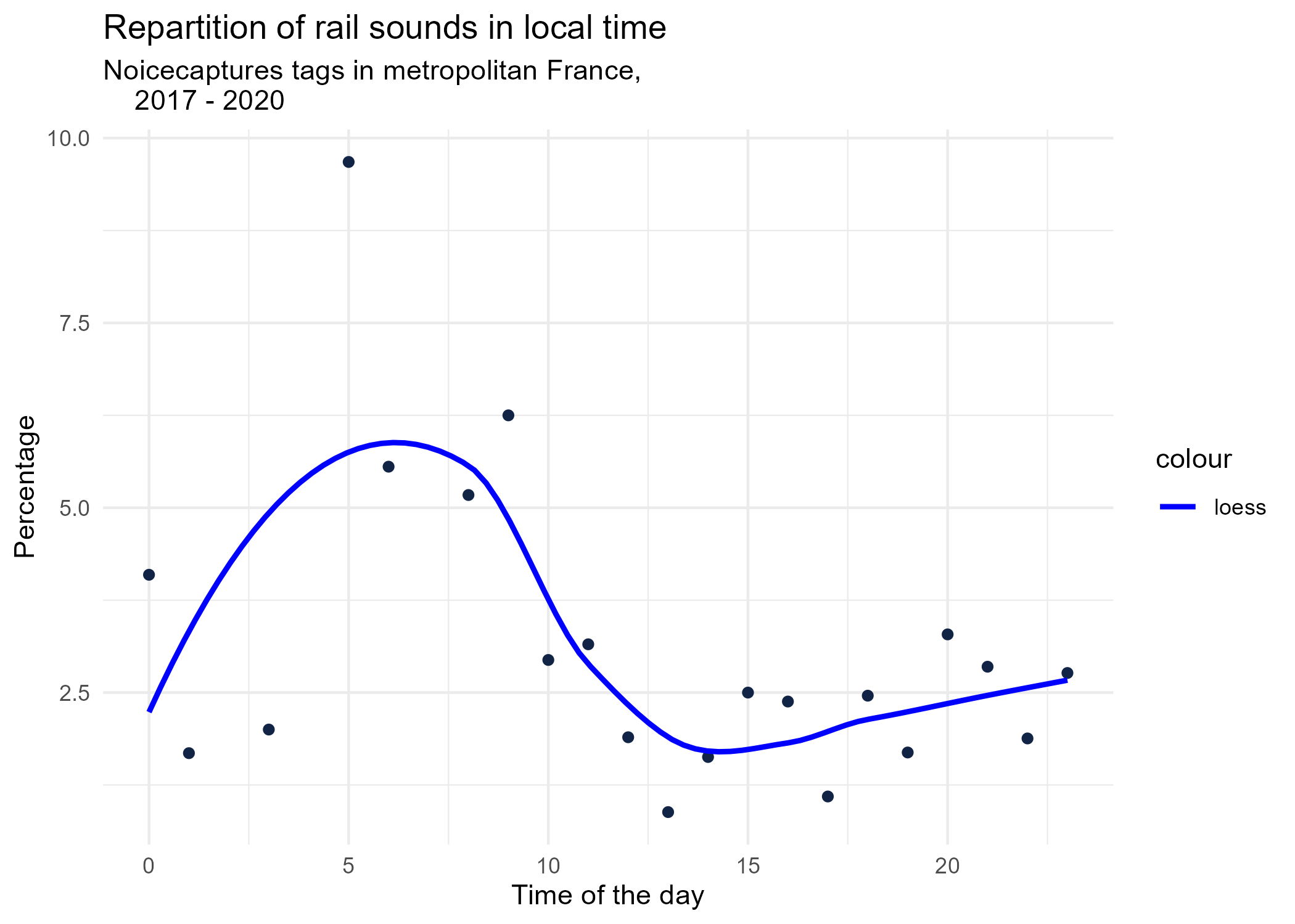
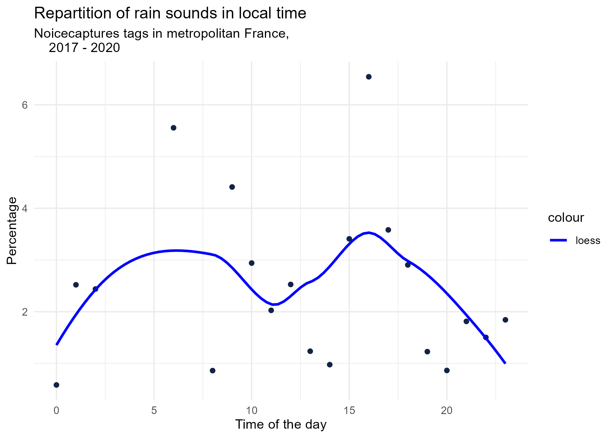
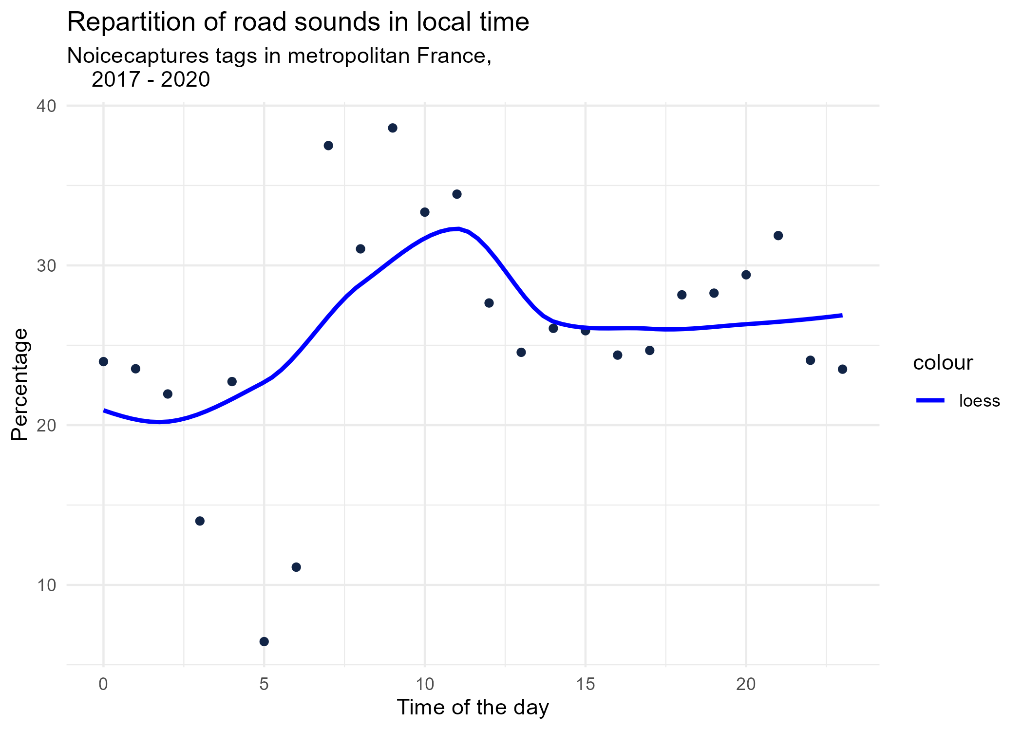
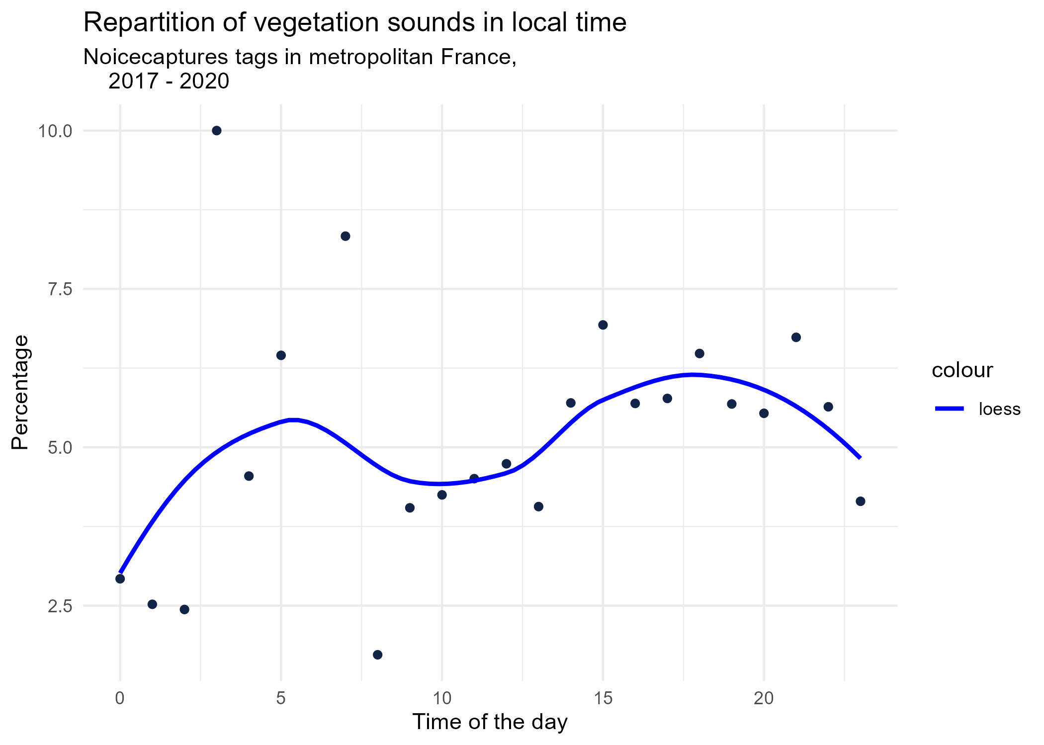
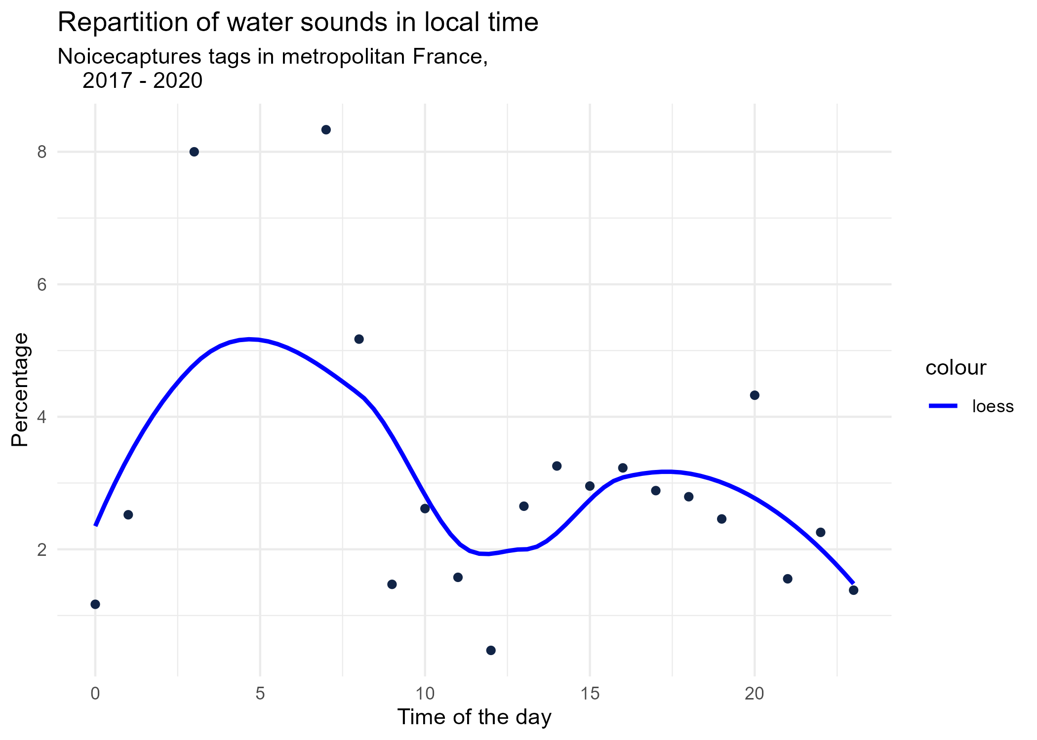
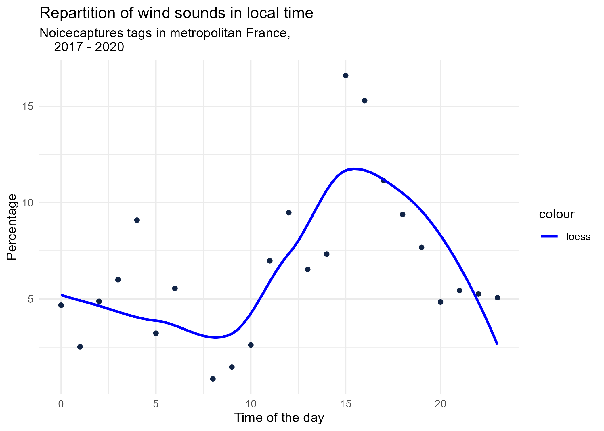
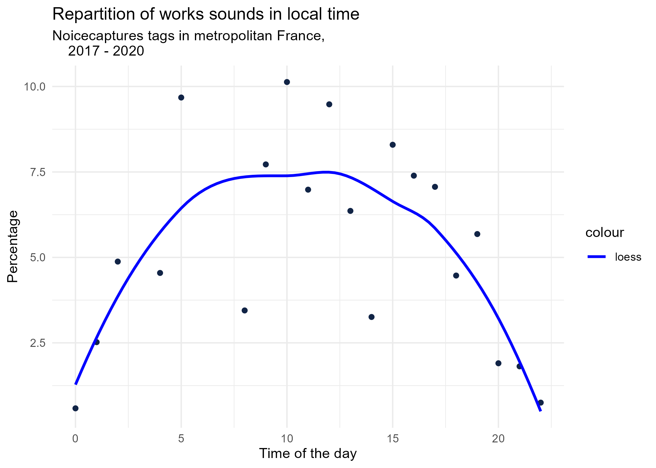
3.1.1 Hourly dynamics, details

dynamic_graphs <- function(tag) {
  
  title <- paste("Repartition of",gsub("_", " ",tag),"sounds in local time")
  ggplot(tags_hourly_repartition %>% dplyr::filter(tag_name == tag)) +
  aes(x = local_time, y = percentage) +
  geom_point(shape = "circle", size = 1.5, colour = "#112446") +
  labs(
    x = "Time of the day",
    y = "Percentage",
    title = title,
    subtitle = "Noicecaptures tags in metropolitan France,
    2017 - 2020"
  ) +
   geom_smooth(method = "loess", se = FALSE, aes(colour="loess")) + # smooth curve test (see span parameter to fit more to the peak before sunrise)
  scale_colour_manual(values=c("blue", "red"))+
   theme_minimal()
  
  # save graphs
  ggsave(paste0("plots/",gsub(" ", "_",title),".png")) 
}

# Render graphs
graphs <- purrr::map(unique(tags_hourly_repartition$tag_name), dynamic_graphs)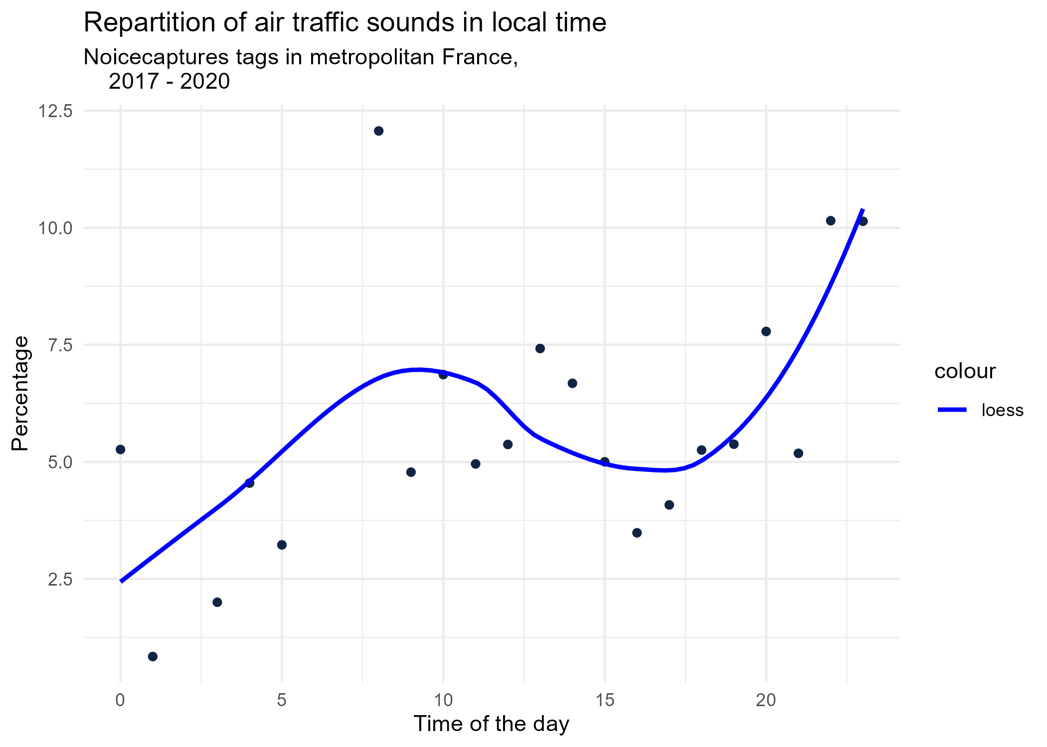

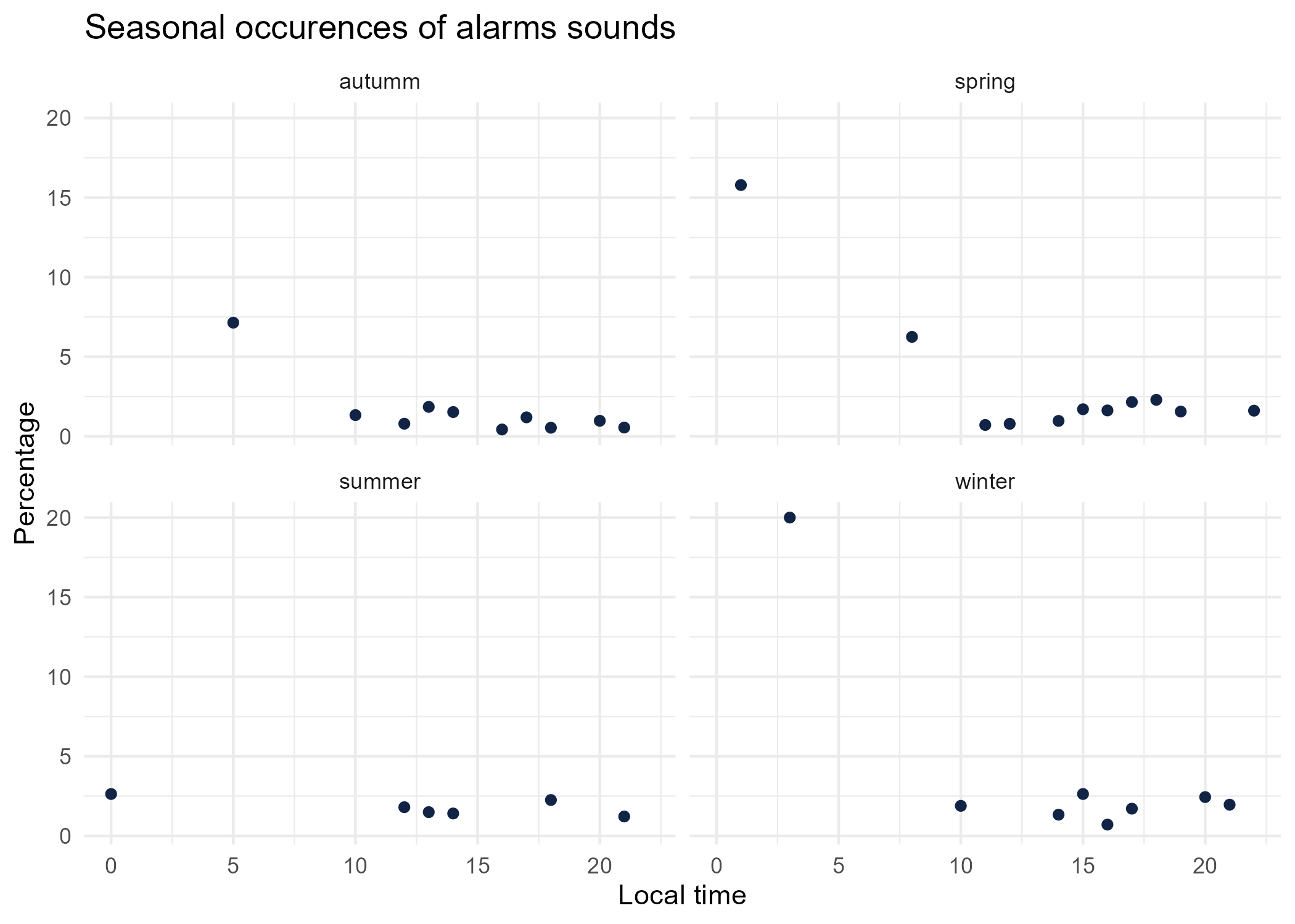
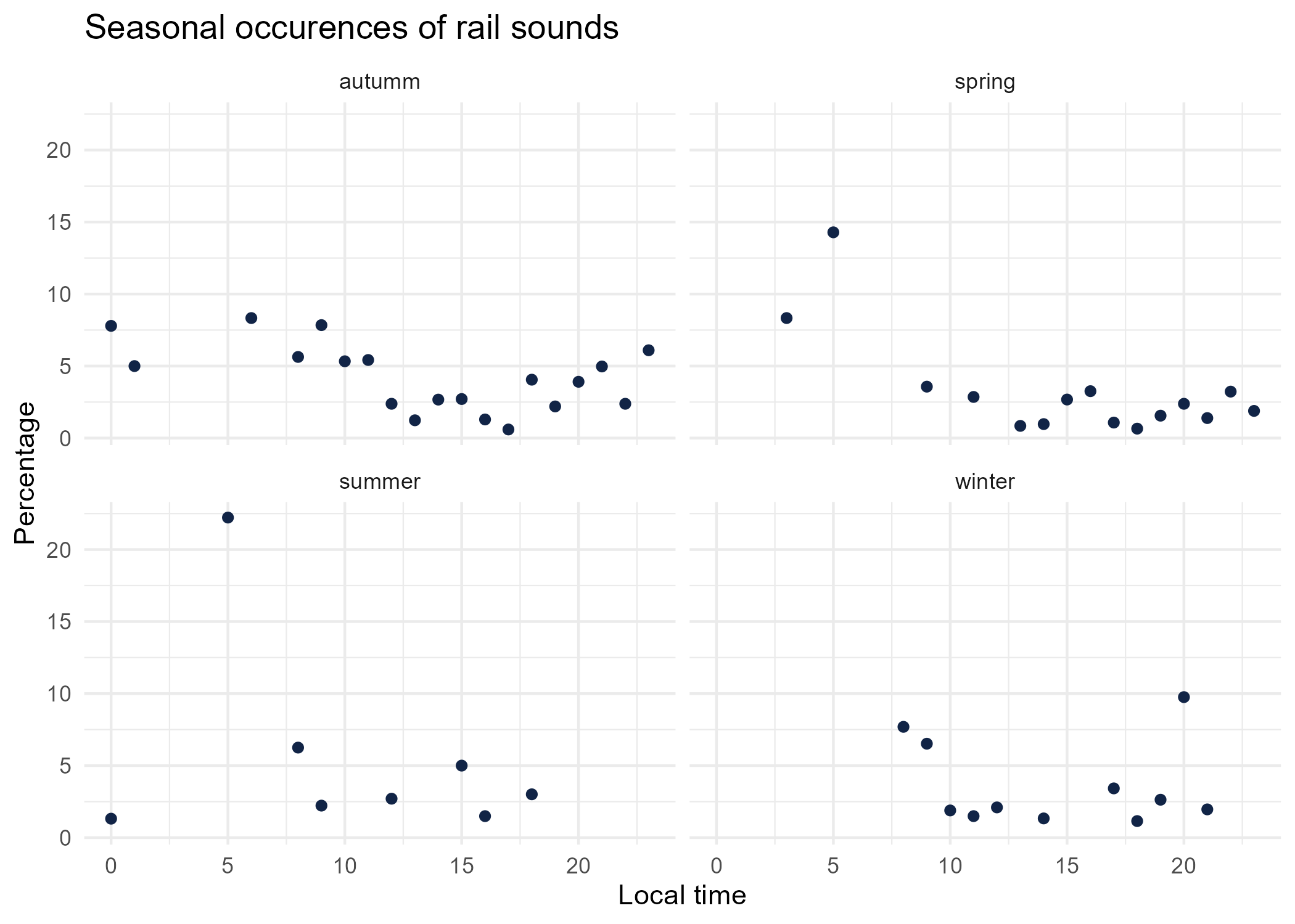
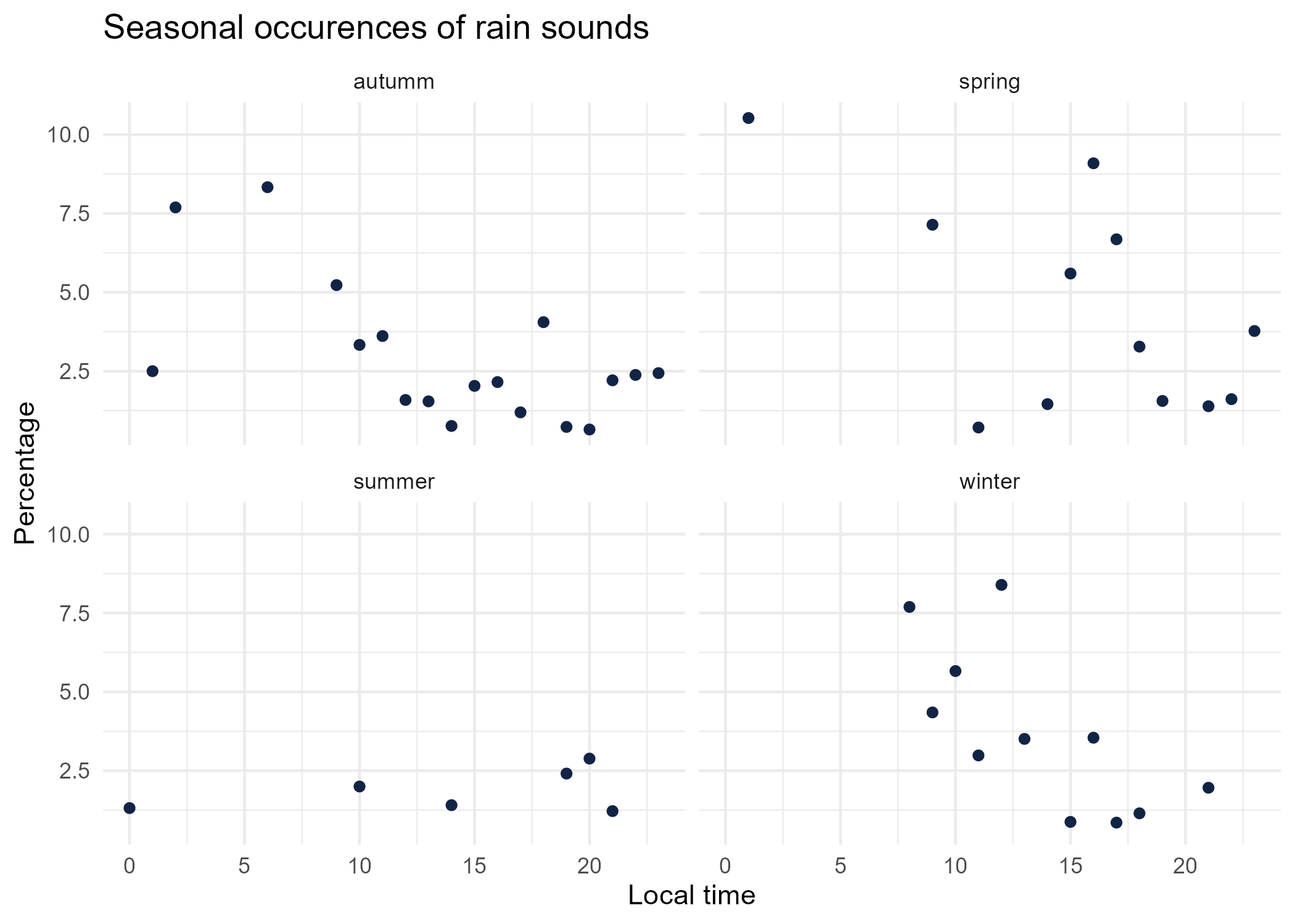
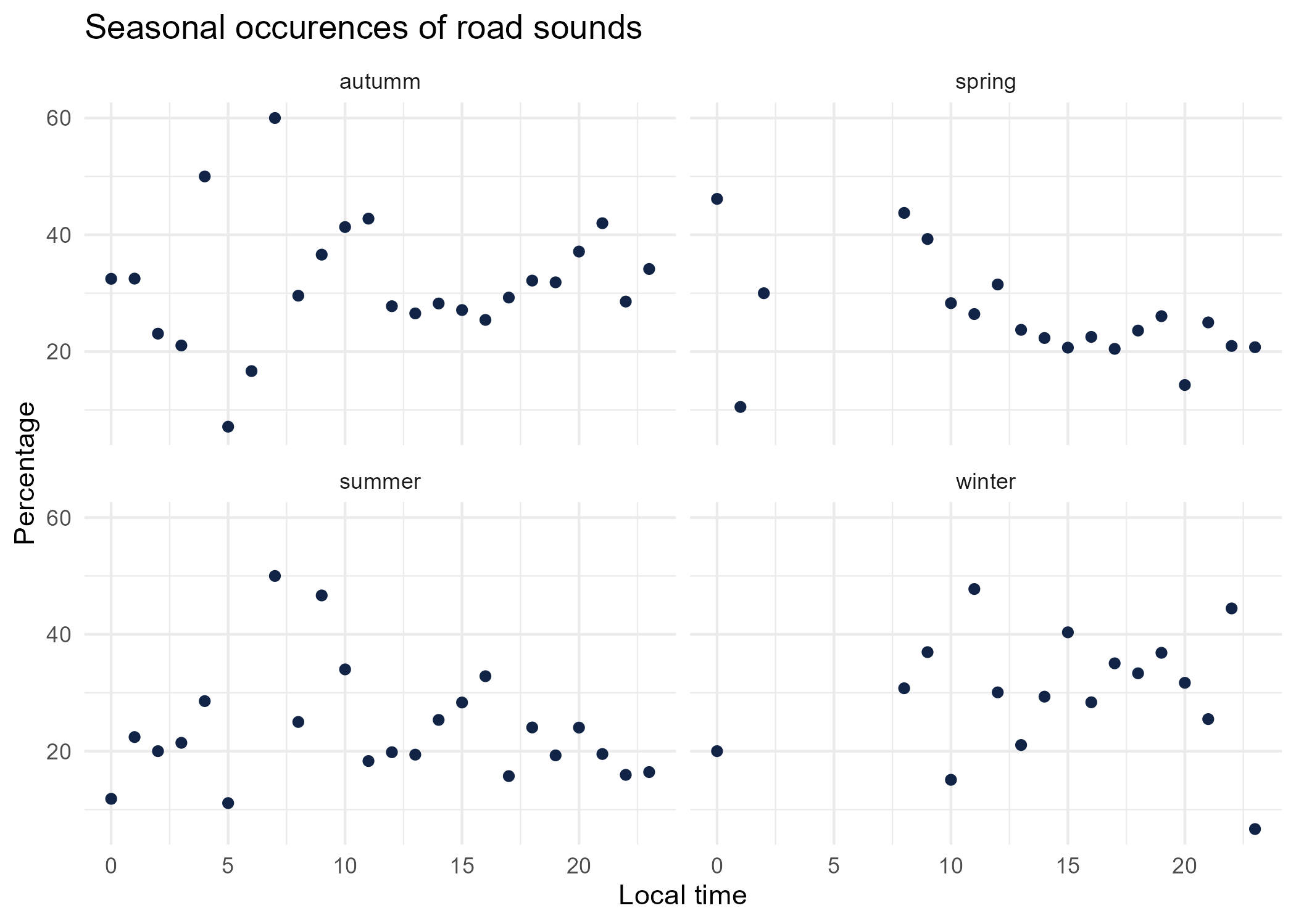
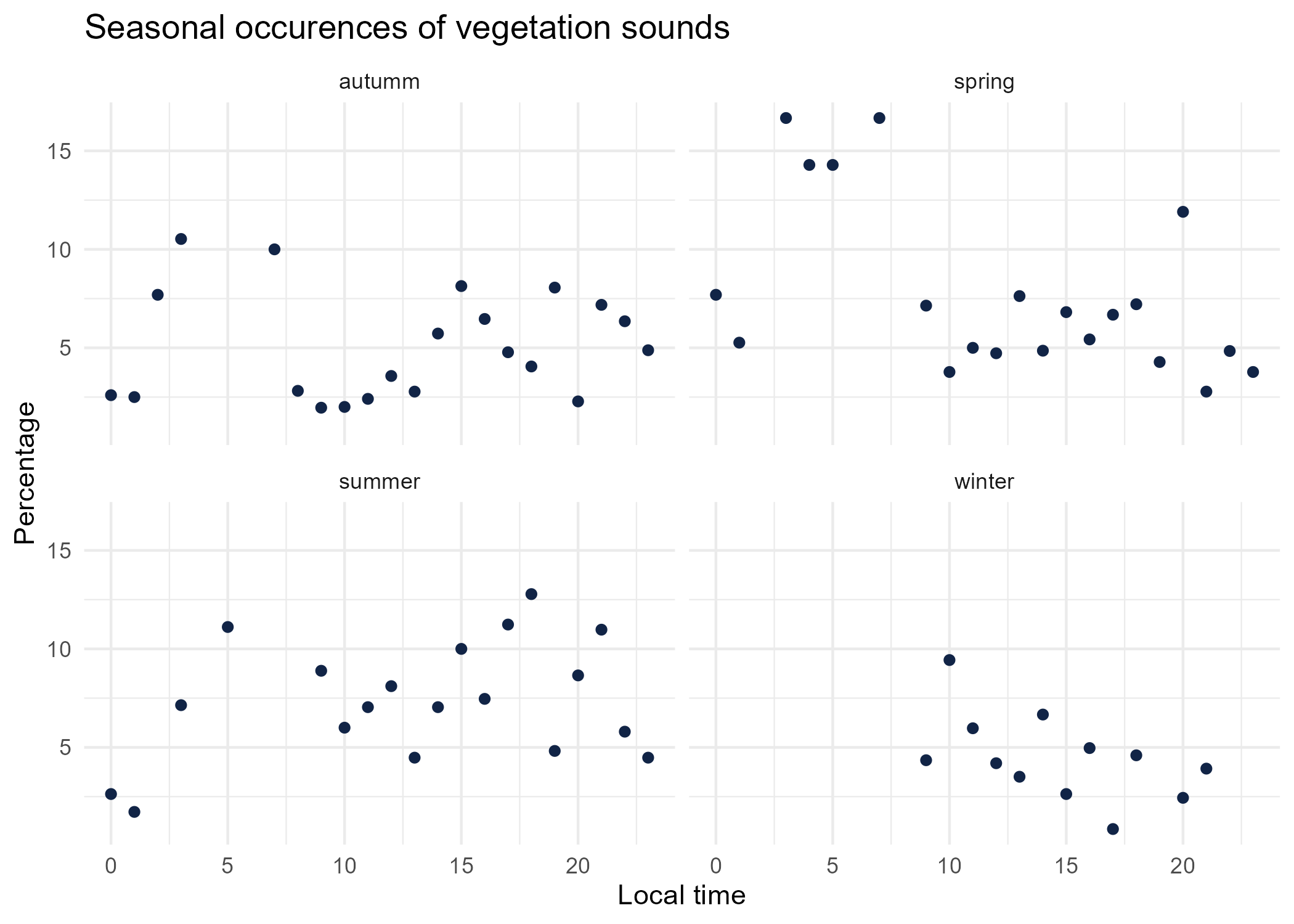
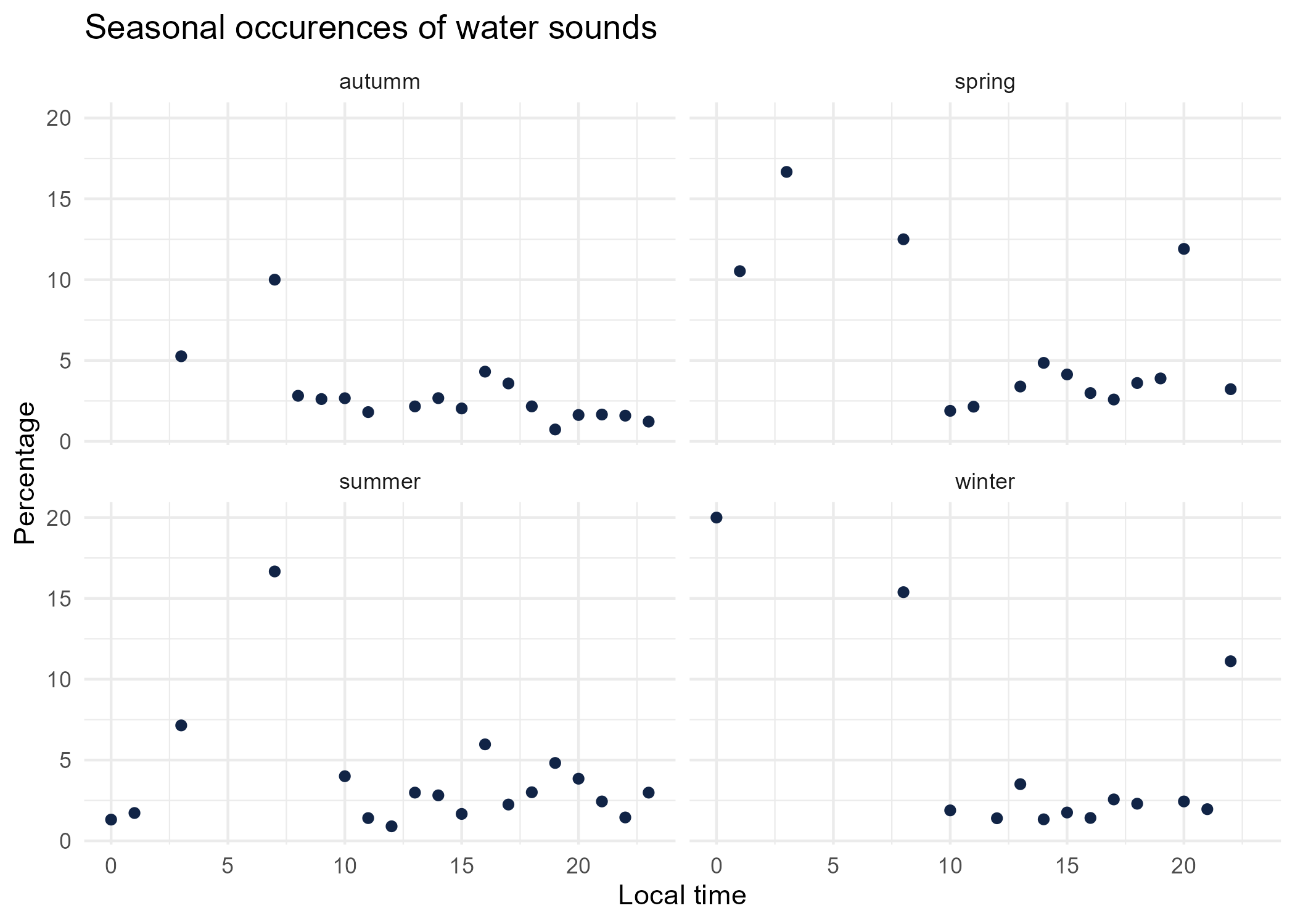
3.2 Seasonal repartition

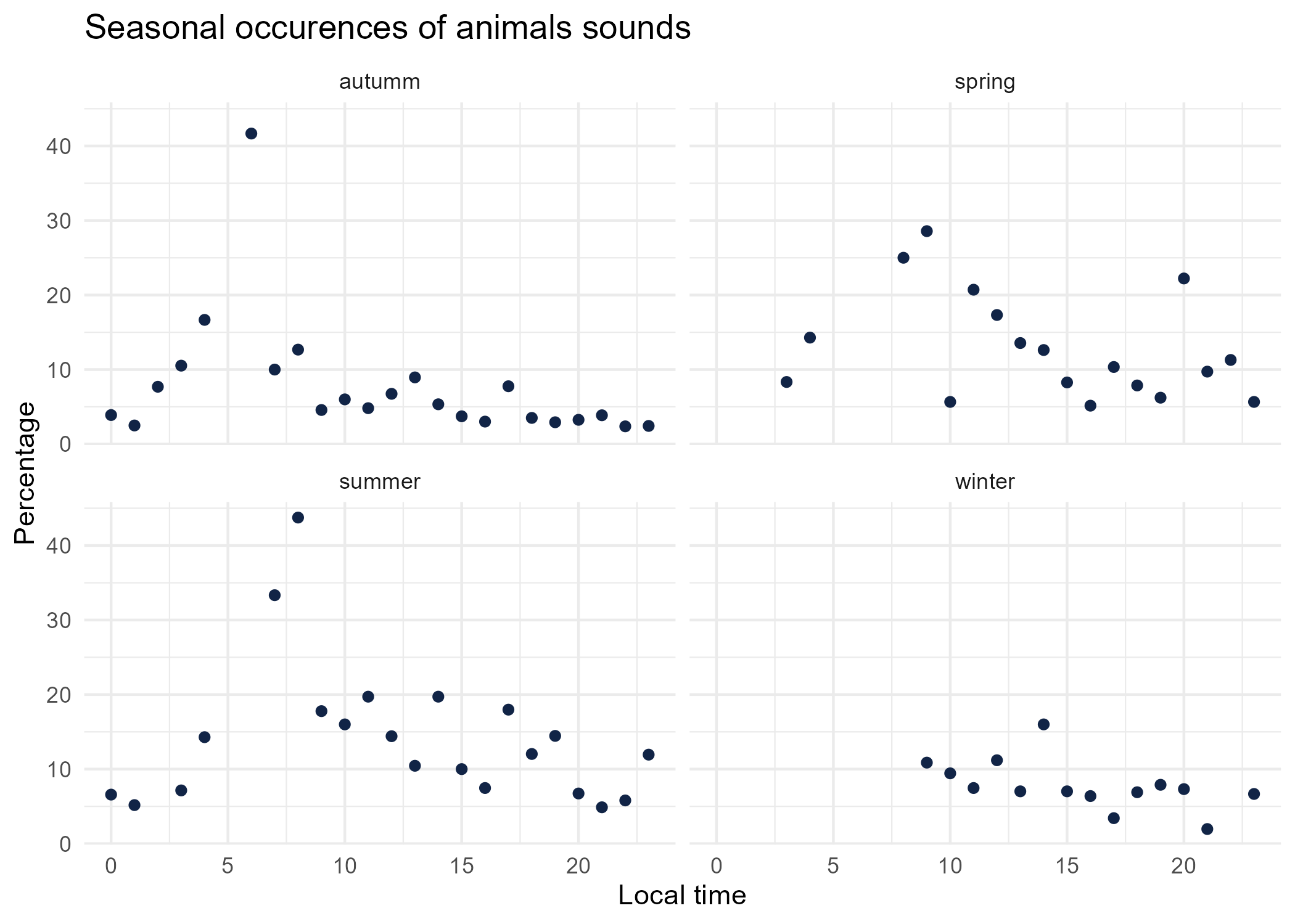
3.2.1 Animals

seasonal_occurences <- all_info %>% 
  dplyr::group_by(tag_name, local_time, season) %>% 
  dplyr::count(name = "occurences")

animals_seasonal_repartition <- seasonal_occurences %>% 
  dplyr::filter(tag_name == "animals") %>% 
  mutate(seasonal_time = paste0(season,'_',local_time)) %>%
  left_join(
    seasonal_occurences %>%
      dplyr::group_by(local_time, season) %>% 
      dplyr::summarise(total = sum(occurences))%>% 
      dplyr::mutate(seasonal_time = paste0(season,'_',local_time)) %>% select(-season),
    by = "seasonal_time") %>% 
  mutate(percentage = occurences * 100 / total)

## `summarise()` has grouped output by 'local_time'. You can override using the
## `.groups` argument.

animals_seasonal_repartition %>% dplyr::select(-local_time.y, -seasonal_time) %>% head() %>% knitr::kable()

tag_name	local_time.x	season	occurences	total	percentage
animals	0	autumm	3	77	3.896104
animals	0	summer	5	76	6.578947
animals	1	autumm	1	40	2.500000
animals	1	summer	3	58	5.172414
animals	2	autumm	1	13	7.692308
animals	3	autumm	2	19	10.526316

ggplot(animals_seasonal_repartition) +
  aes(x = local_time.x, y = percentage) +
  geom_point(shape = "circle", size = 1.5, colour = "#112446") +
  labs(
    x = "Local time",
    y = "Percentage",
    title = "Seasonal occurences of animals sounds"
  ) +
  theme_minimal() +
  facet_wrap(vars(season))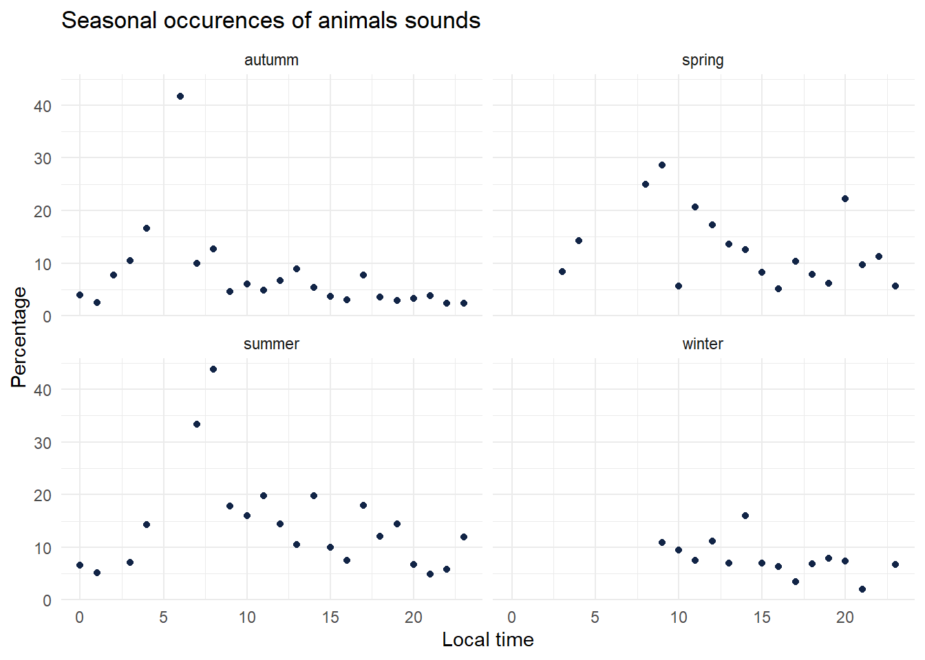

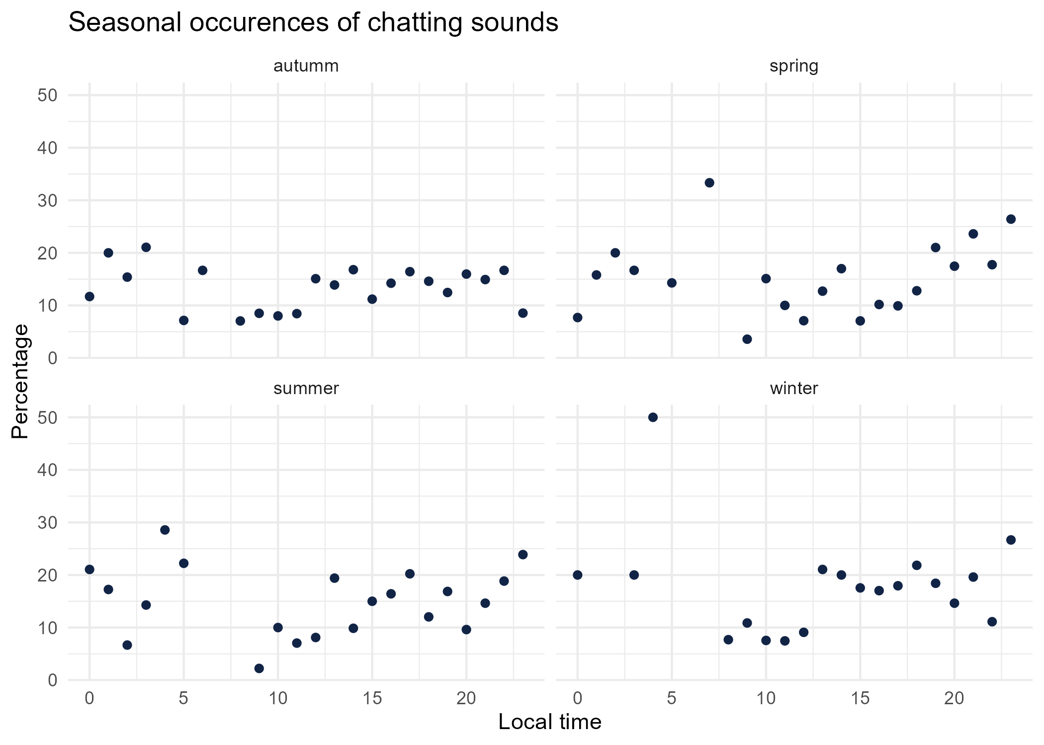
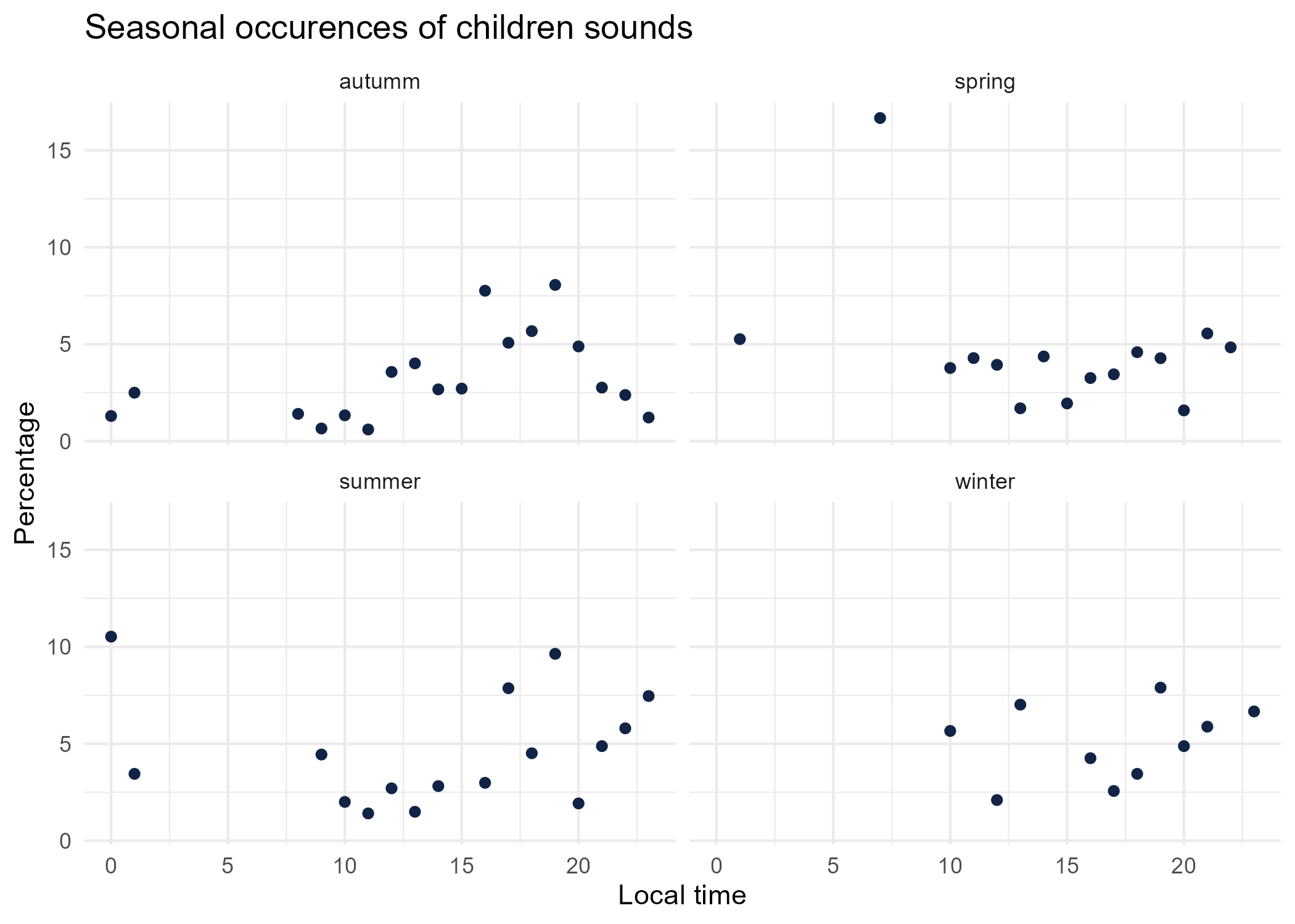
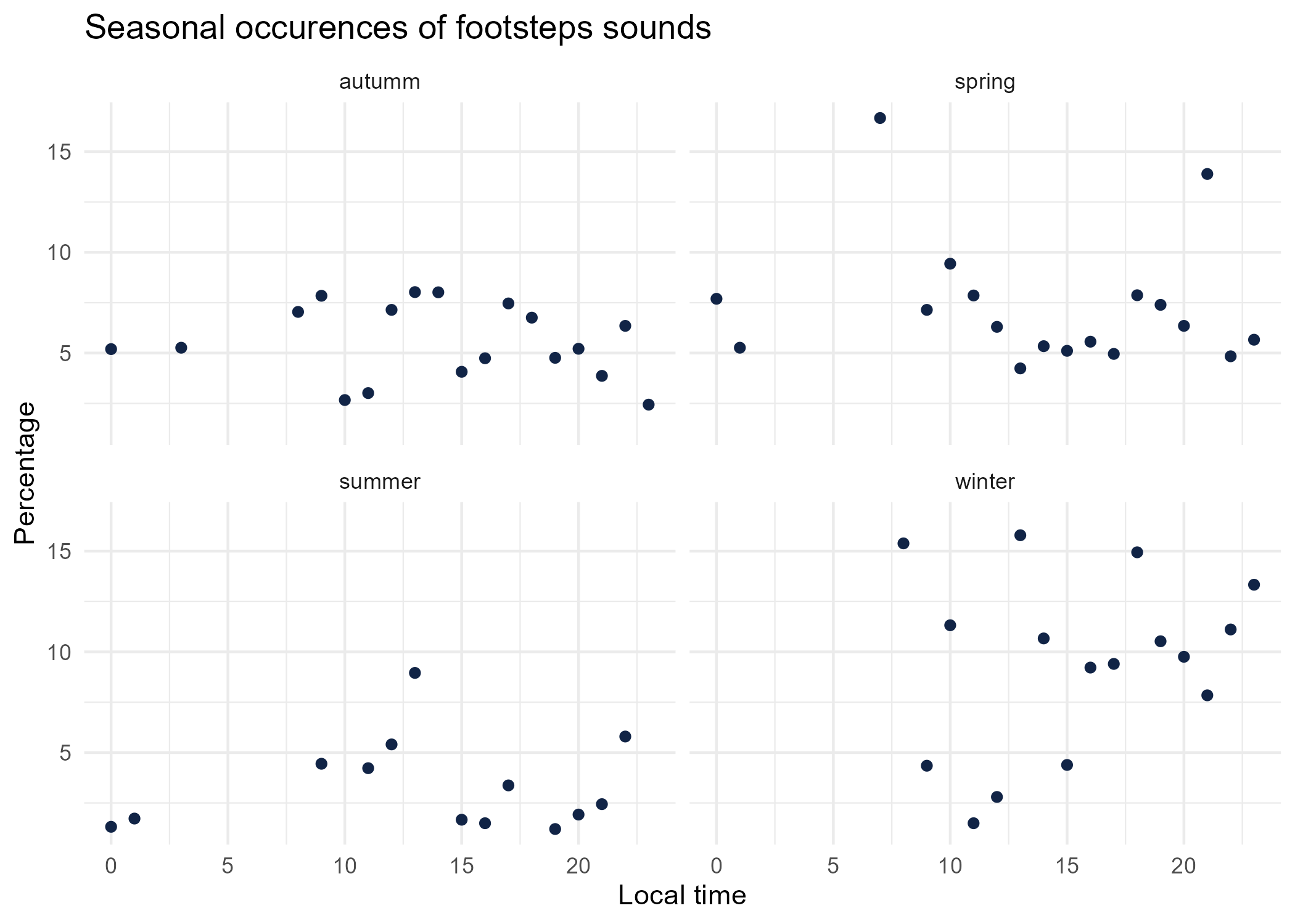
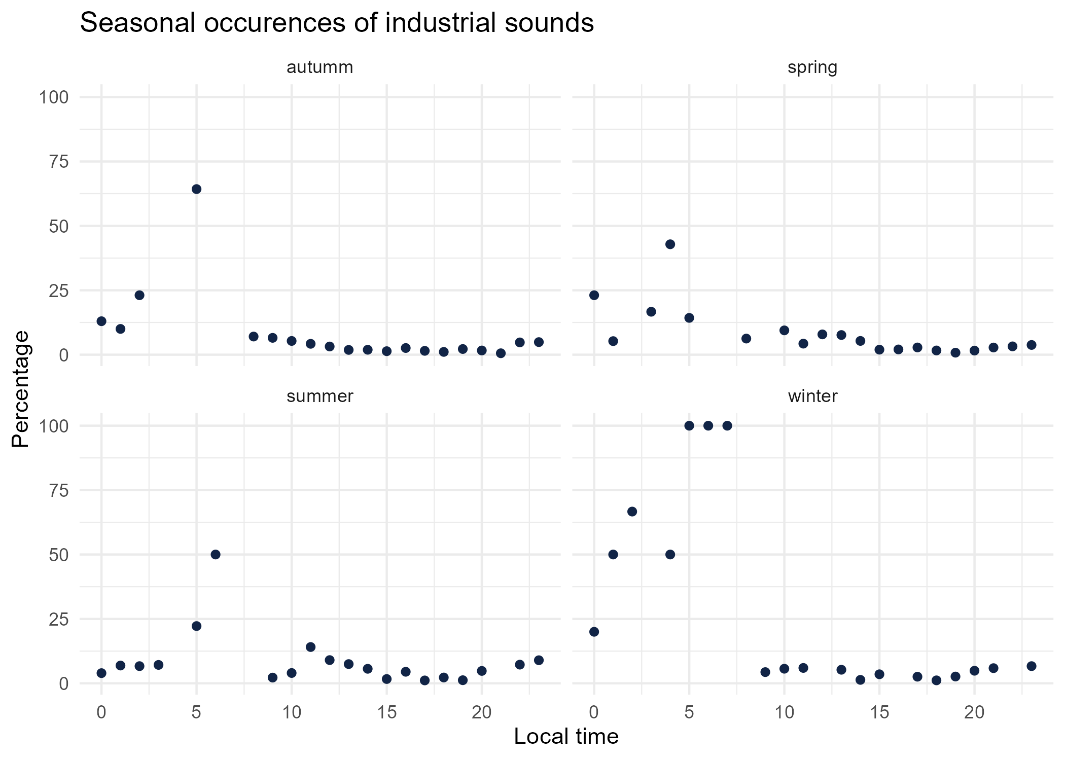
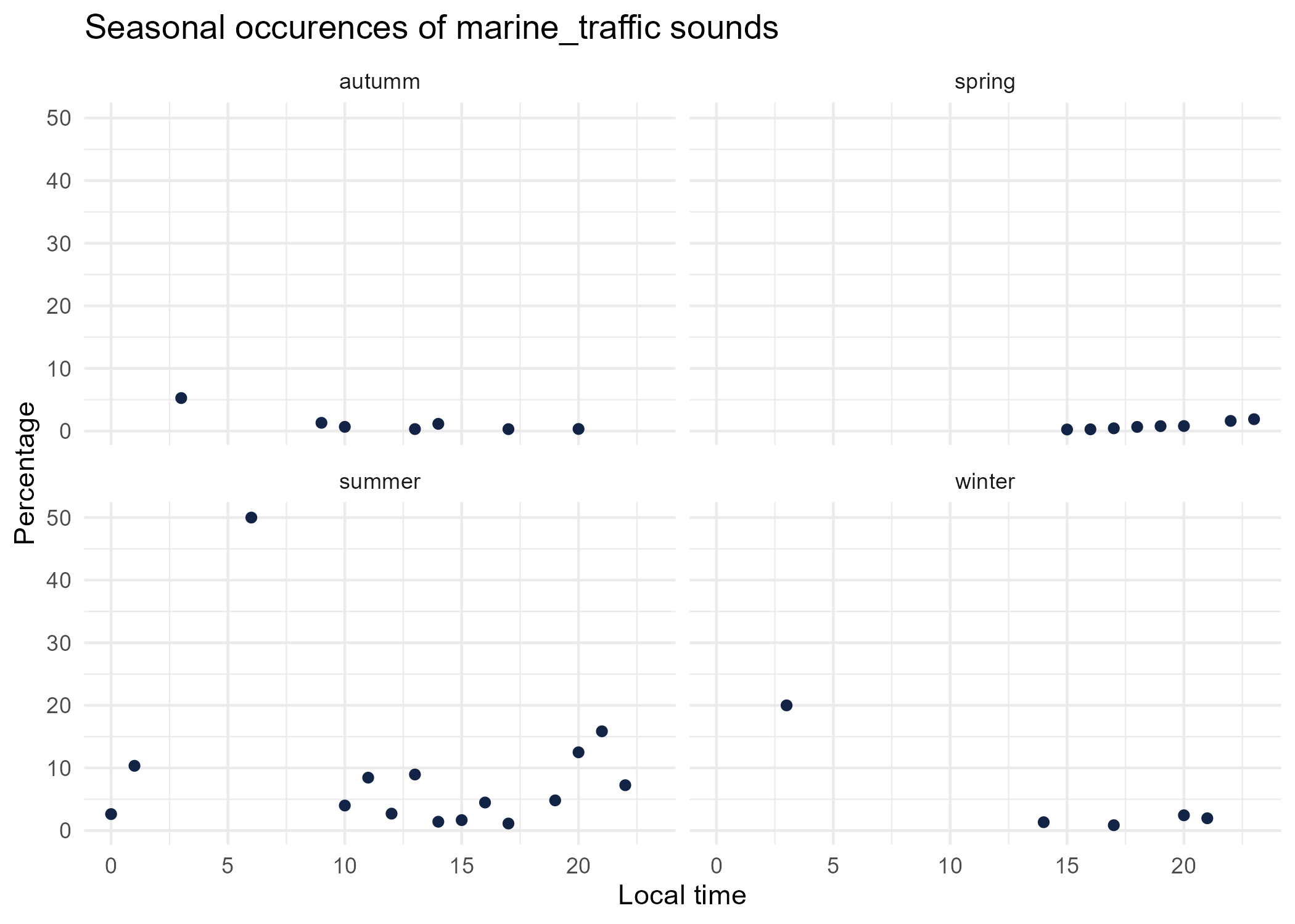
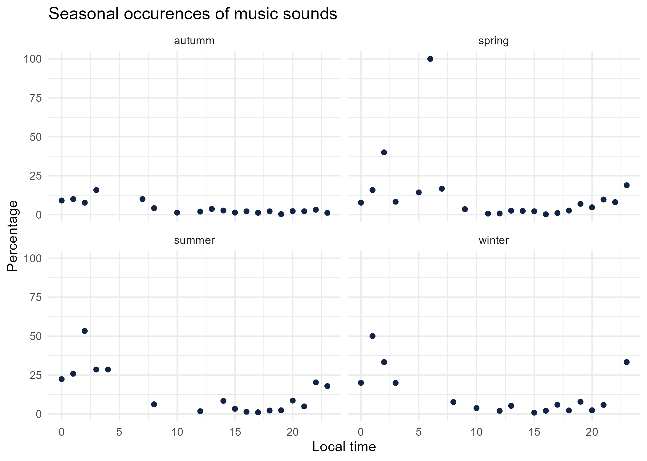
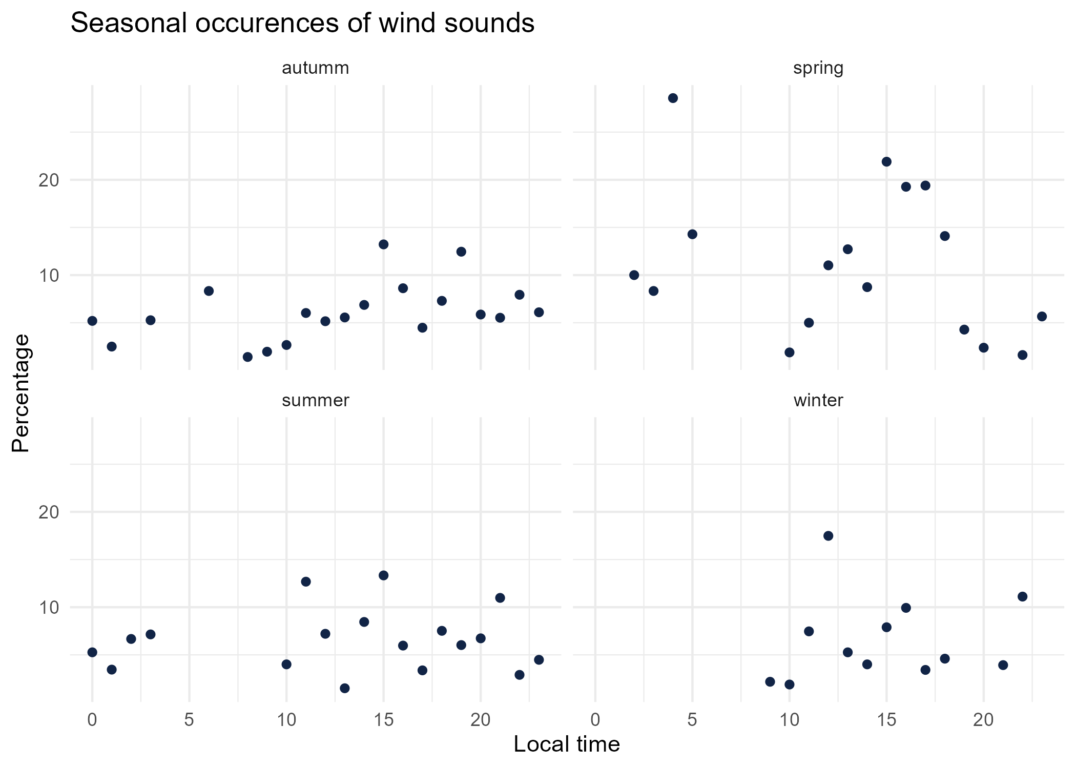
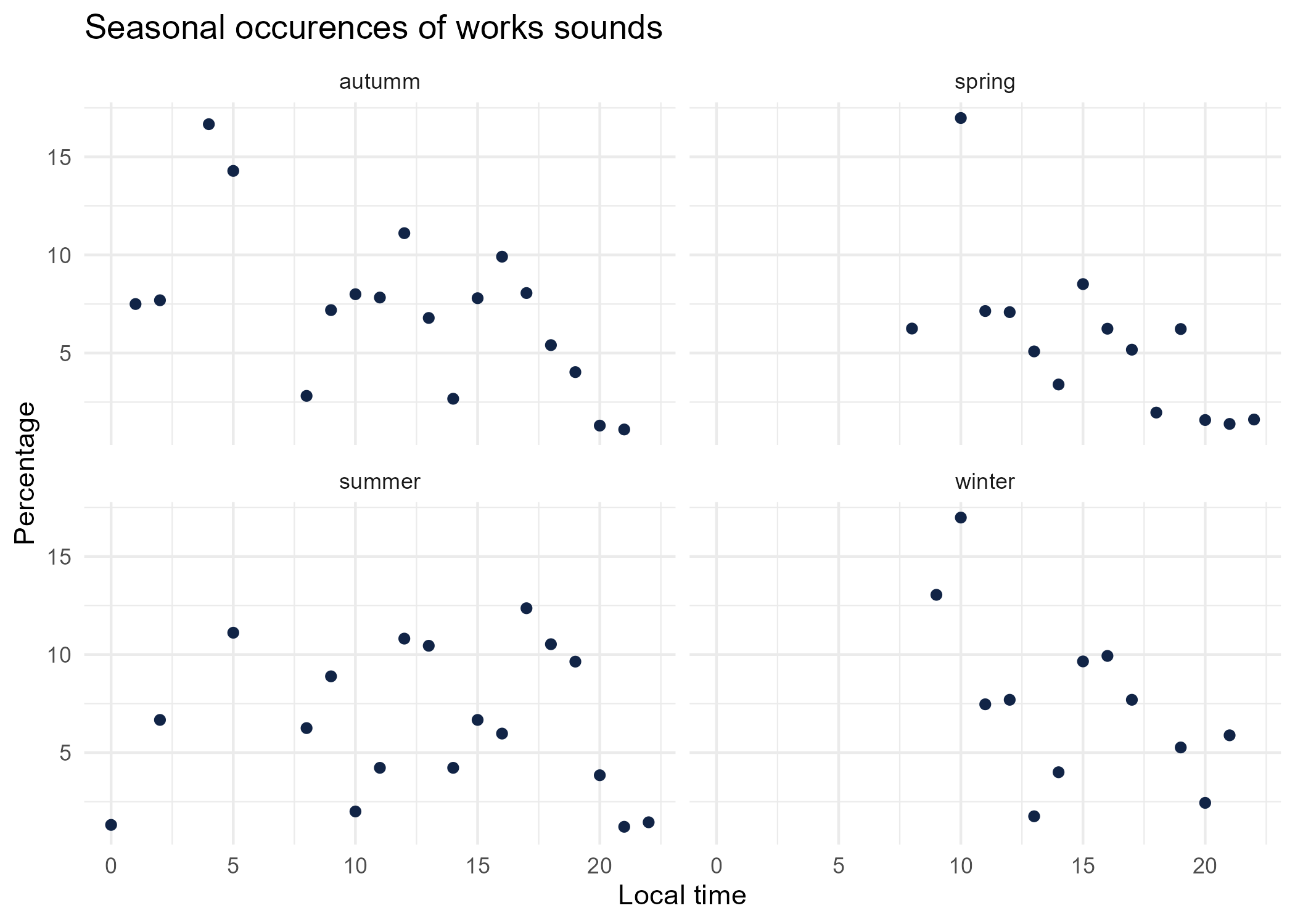
season_graphs <- function(tag) {
  
  title <- paste("Seasonal occurences of",tag,"sounds")
  seasonal_occurences %>% 
  dplyr::filter(tag_name == tag) %>% 
  mutate(seasonal_time = paste0(season,'_',local_time)) %>%
  left_join(
    seasonal_occurences %>%
      dplyr::group_by(local_time, season) %>% 
      dplyr::summarise(total = sum(occurences))%>% 
      dplyr::mutate(seasonal_time = paste0(season,'_',local_time)) %>% select(-season),
    by = "seasonal_time") %>% 
  mutate(percentage = occurences * 100 / total) %>%
    ggplot() +
  aes(x = local_time.x, y = percentage) +
  geom_point(shape = "circle", size = 1.5, colour = "#112446") +
  labs(
    x = "Local time",
    y = "Percentage",
    title = title
  ) +
  theme_minimal() +
  facet_wrap(vars(season))
  
  # save graphs
  ggsave(paste0("plots/",gsub(" ", "_",title),".png")) 
}

# Render graphs
graphs <- purrr::map(unique(seasonal_occurences$tag_name), season_graphs)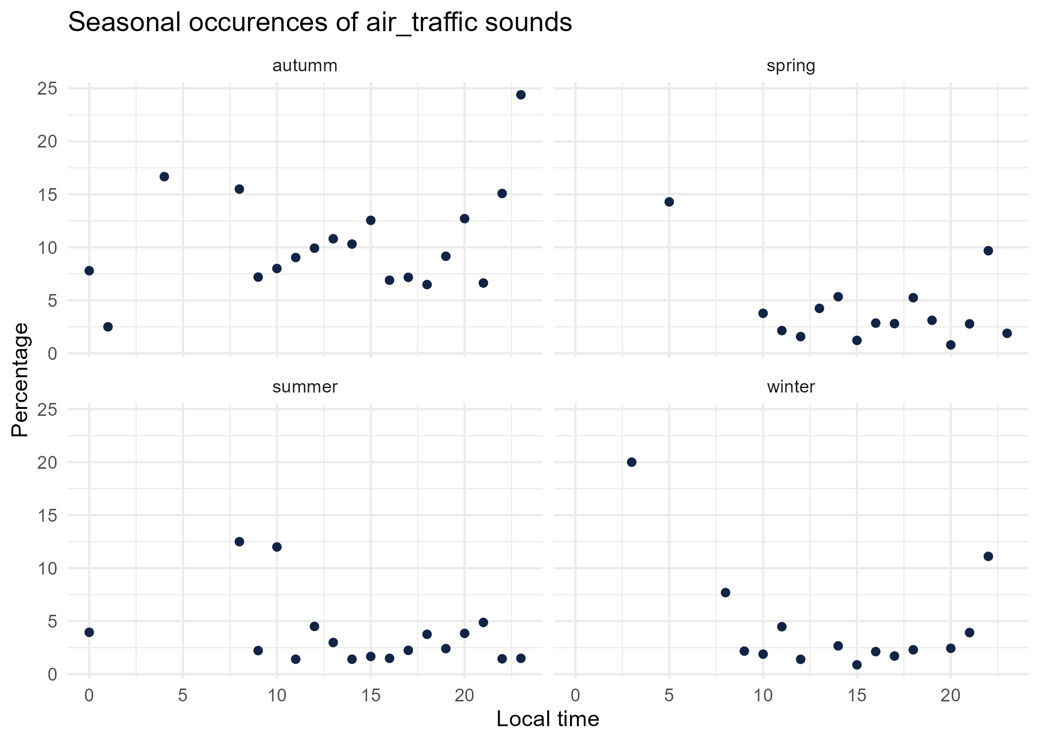

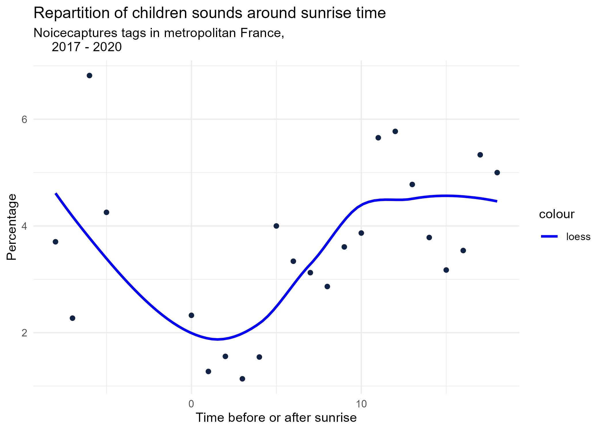
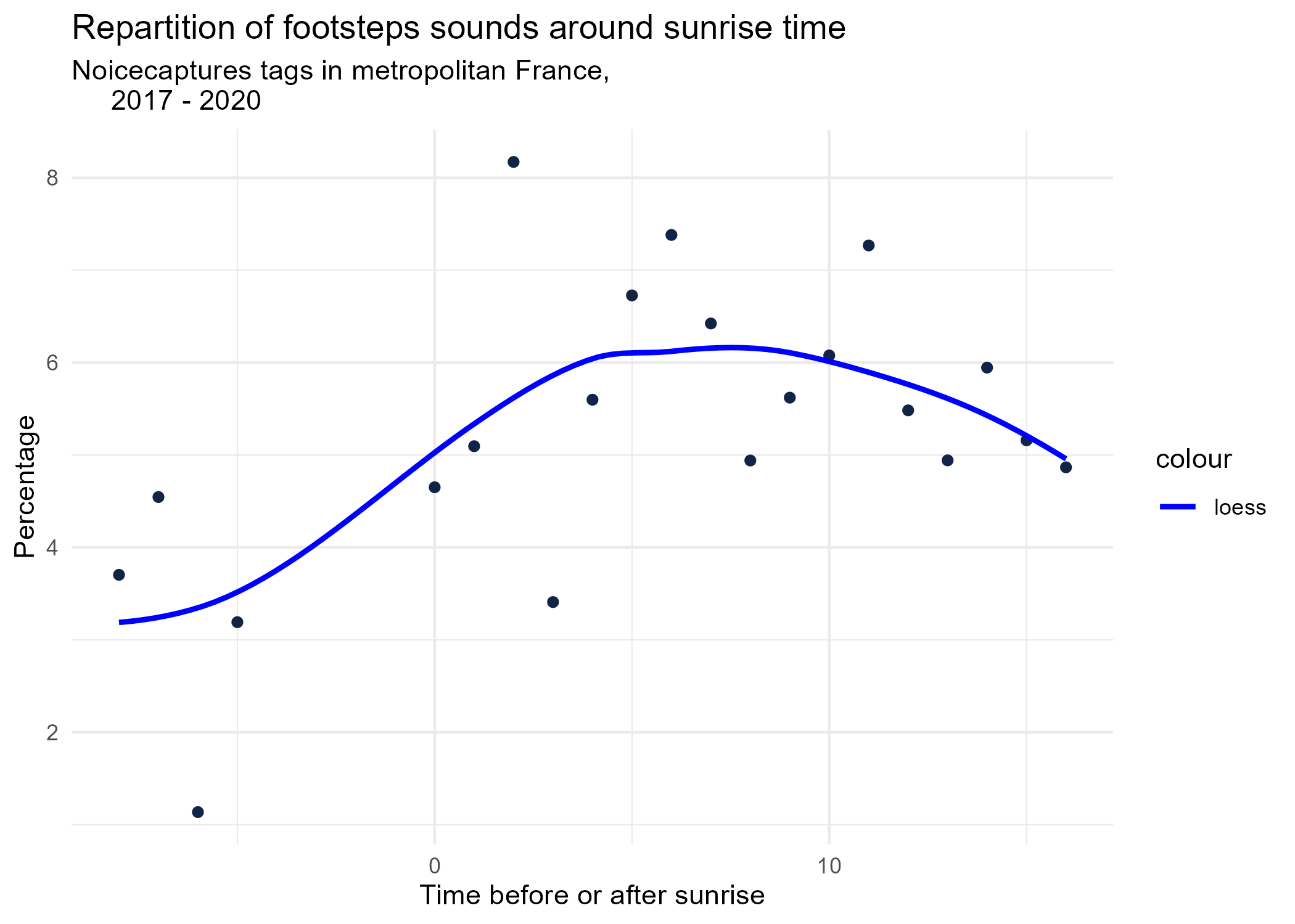
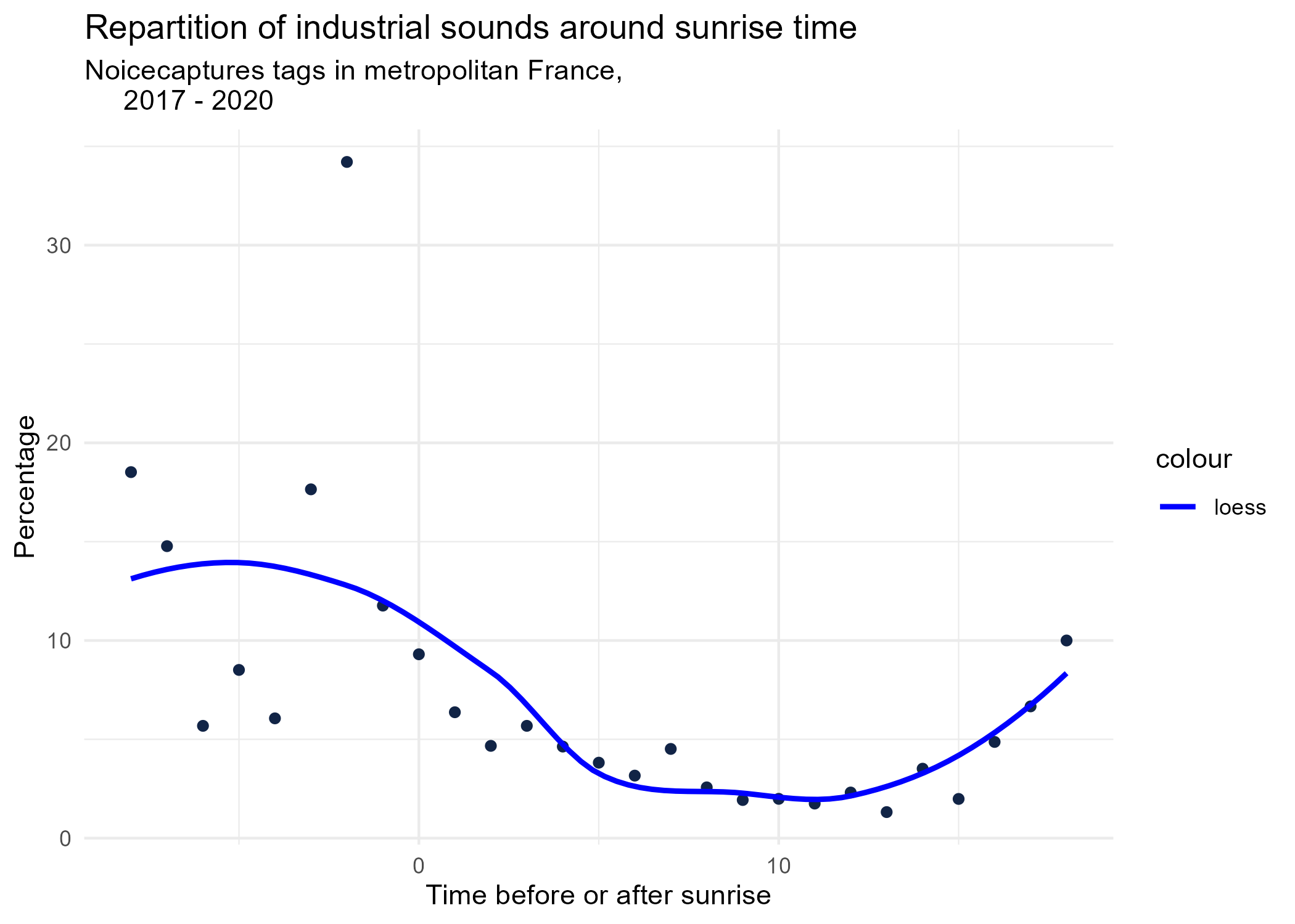
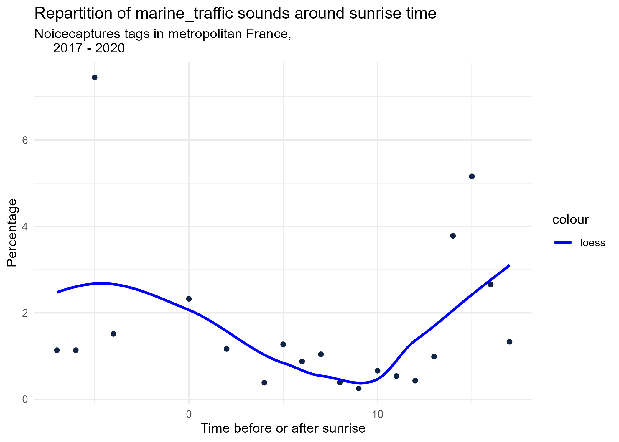
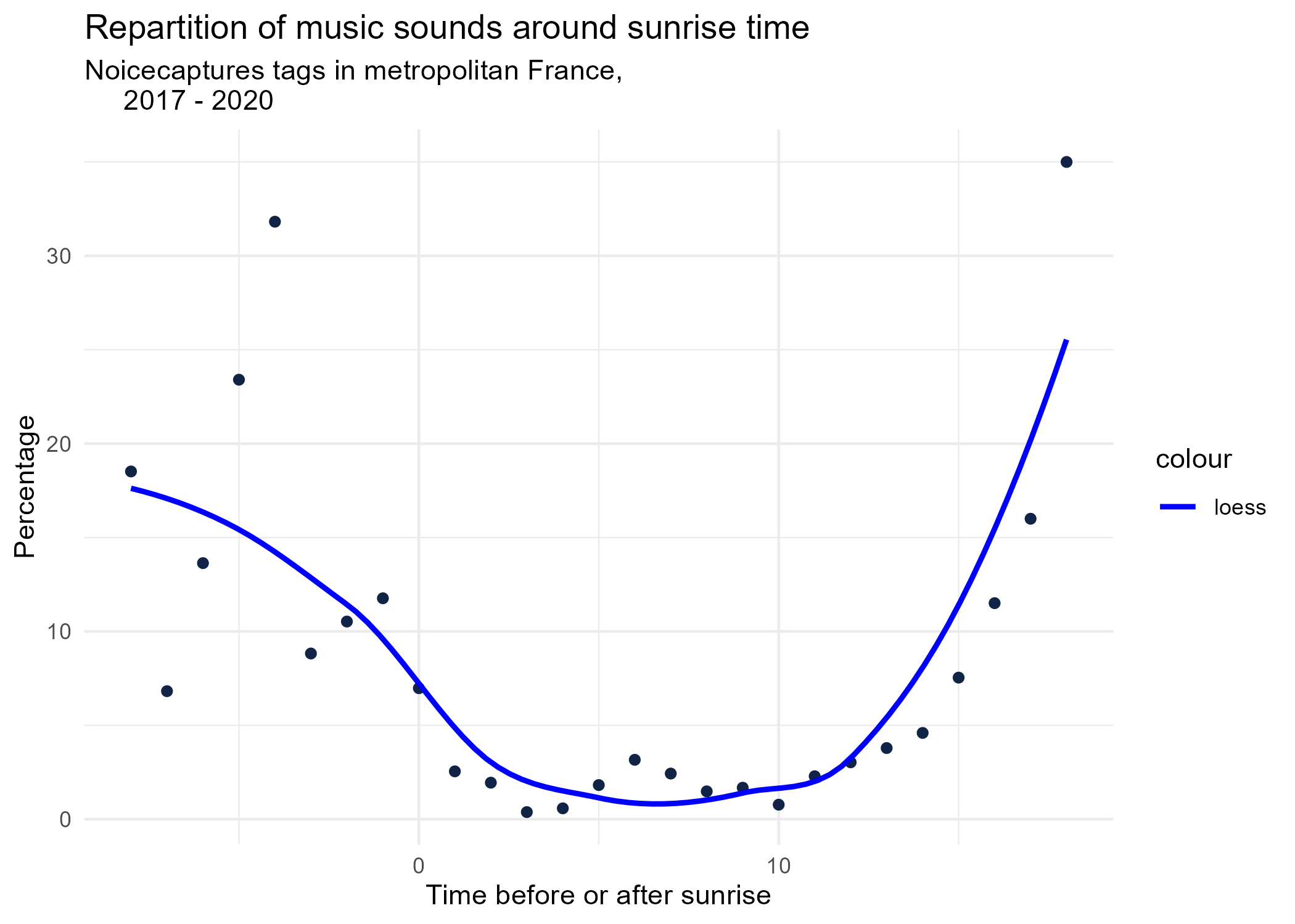
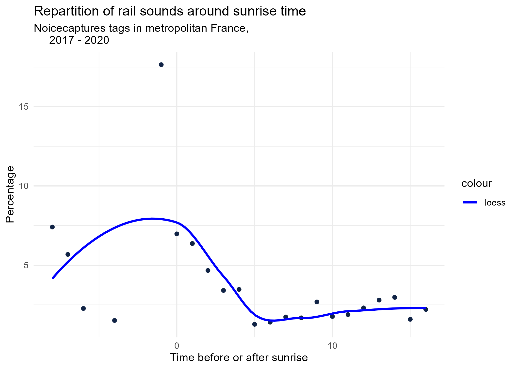
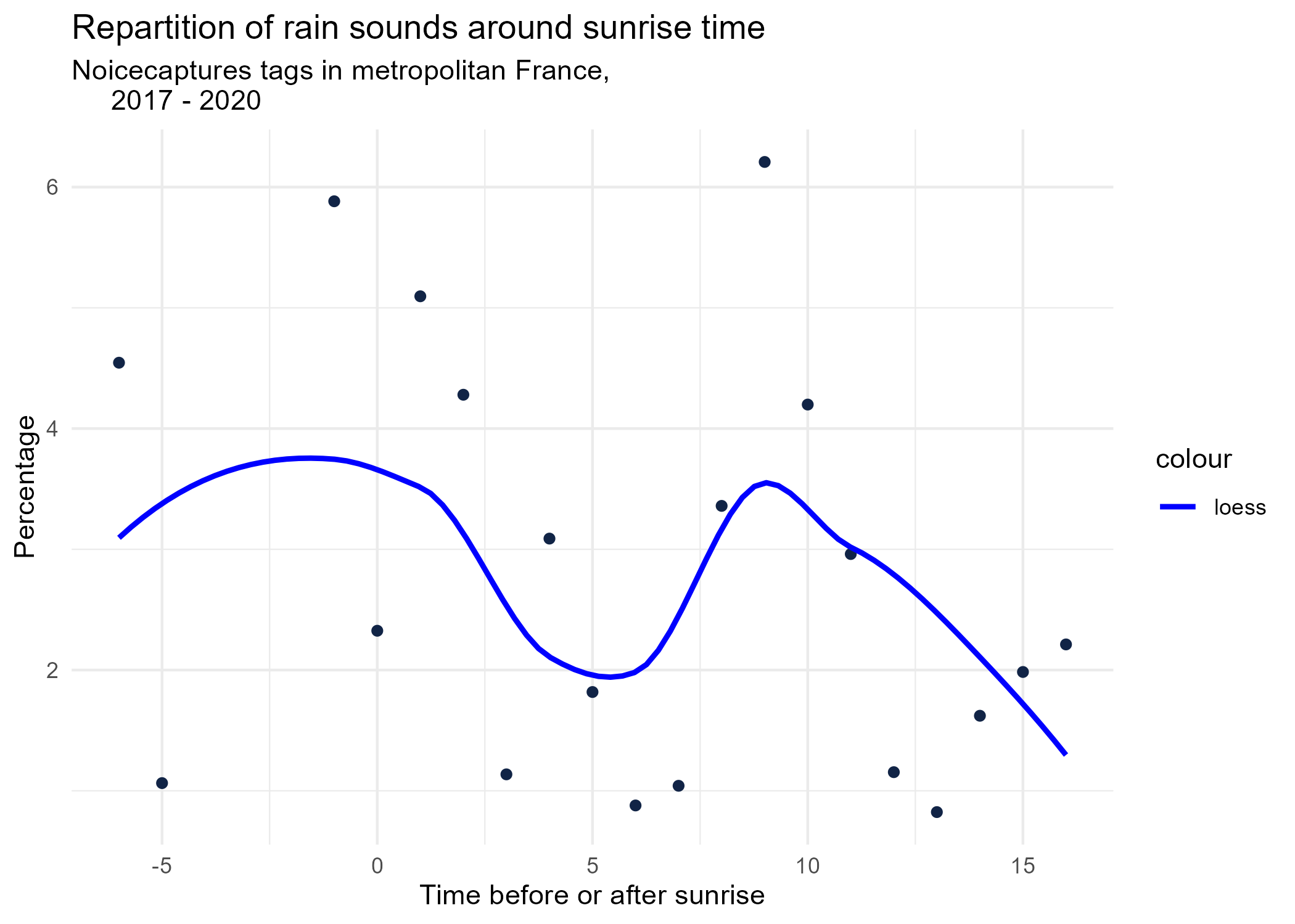
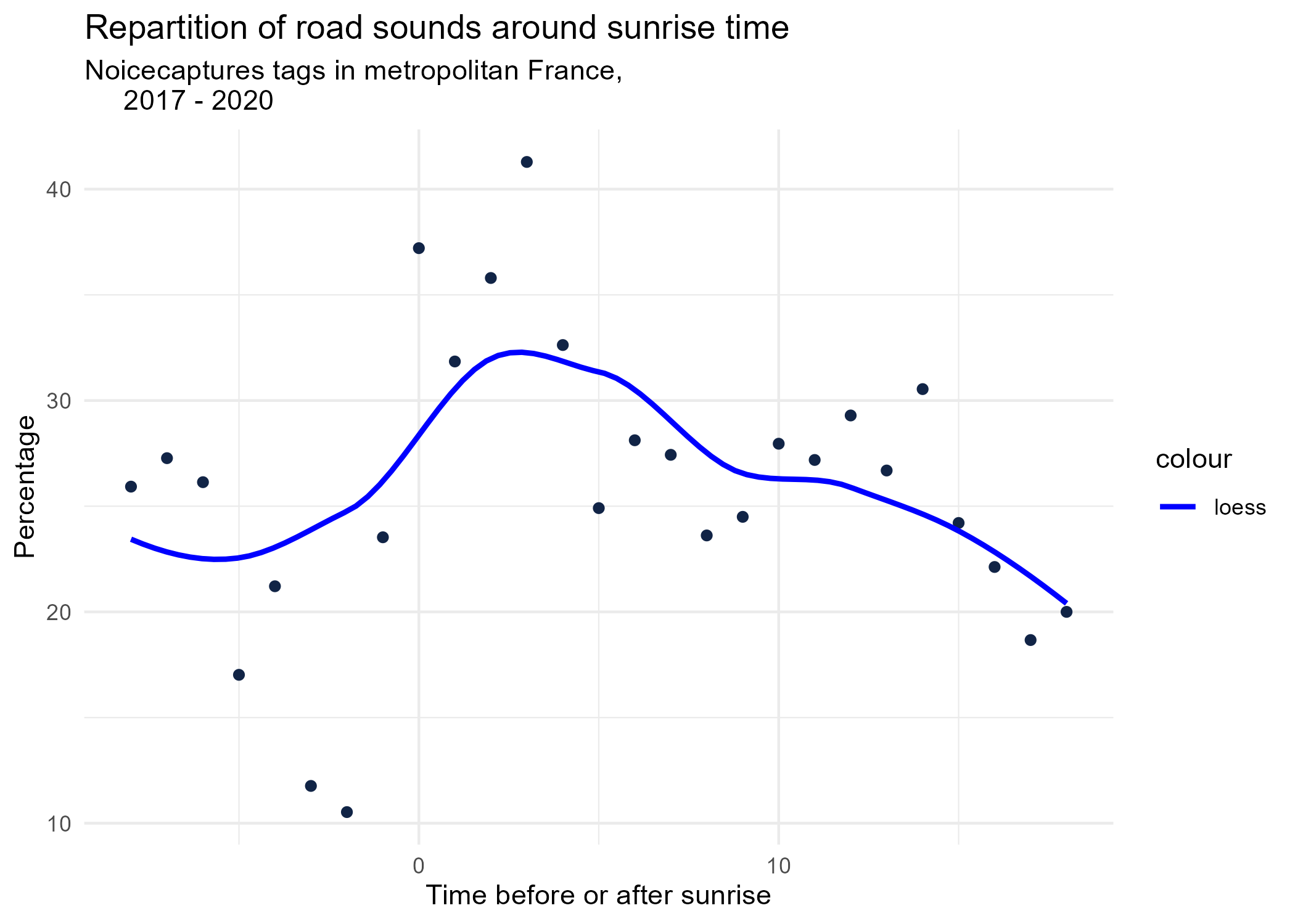
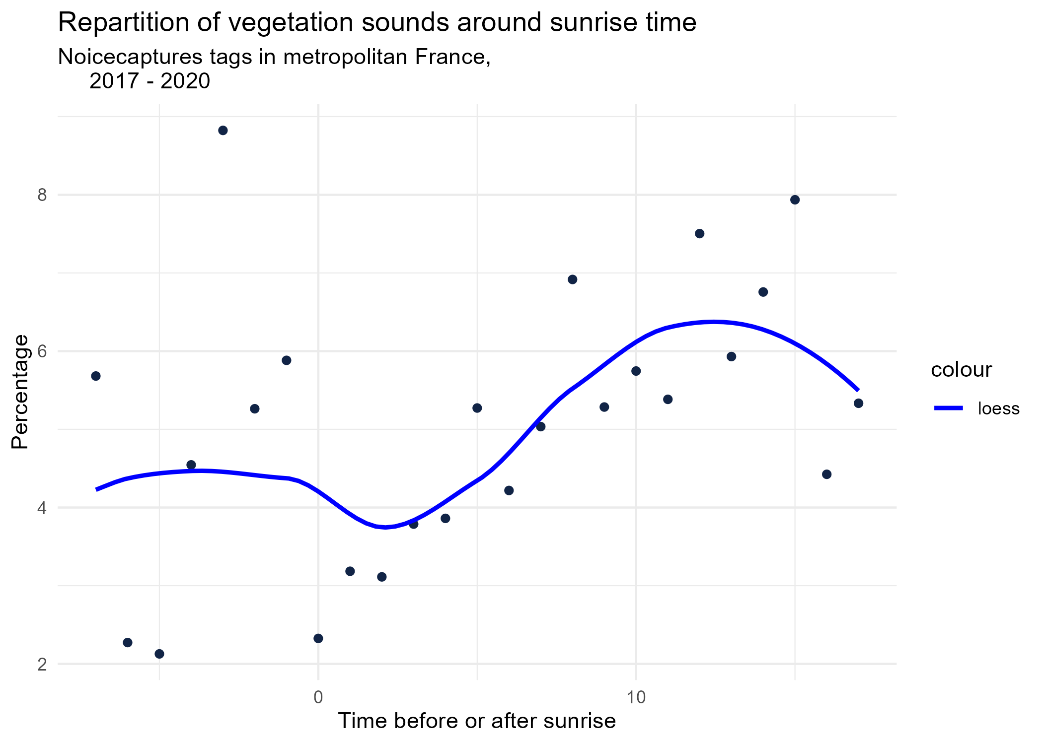
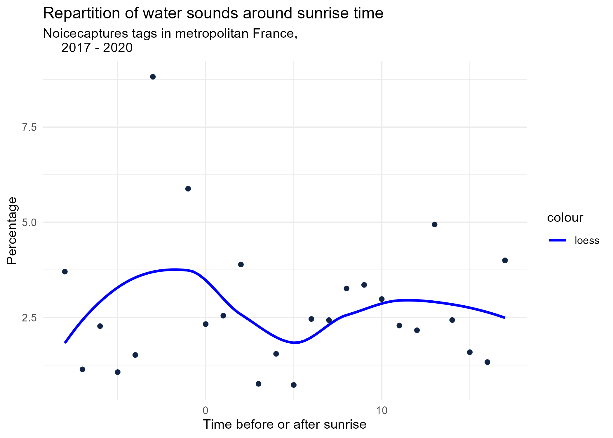
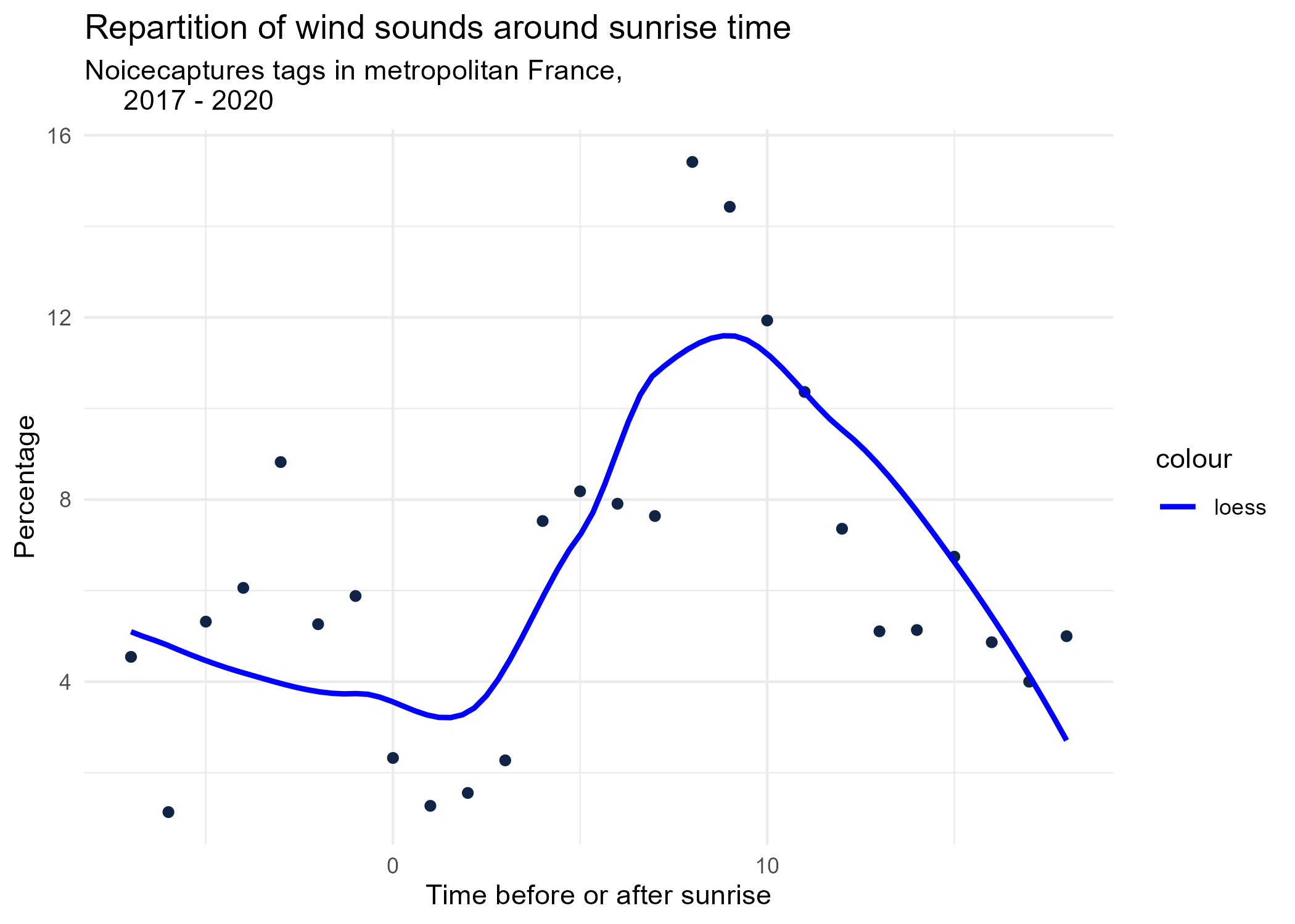
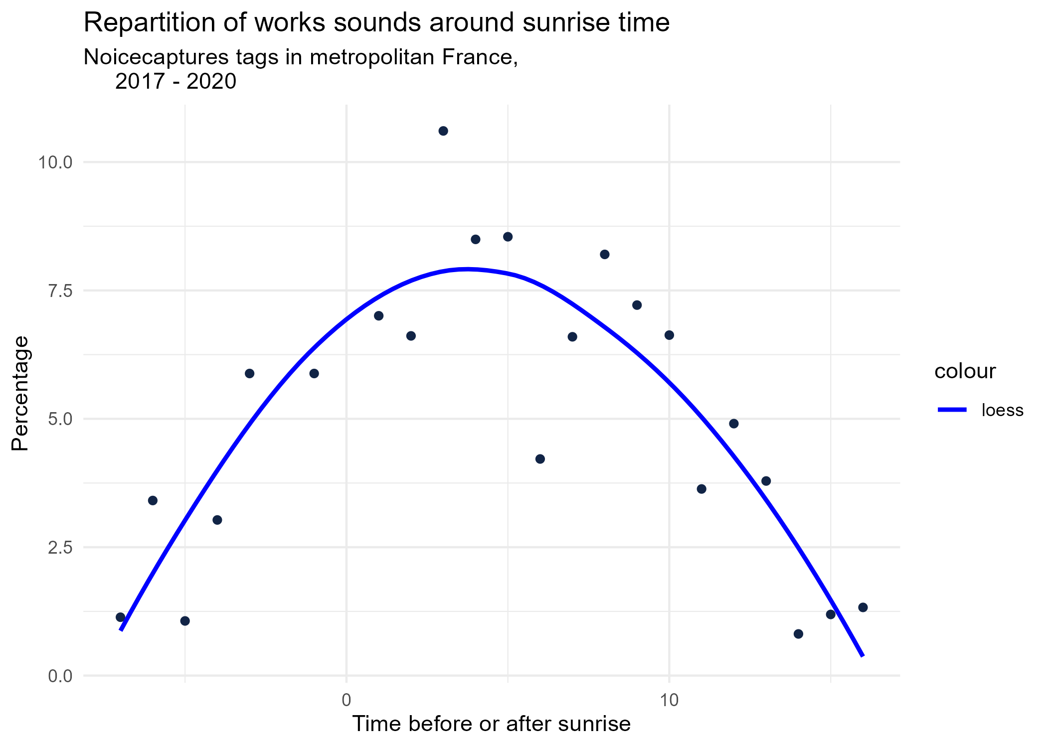
4 Sound dynamics: sunrise study

get_sunrise <- function(pk_track, date, lat, lon, tz ="UTC") {
  # compute sunrise time from localisation and UTC time
  #return NA if error
  in_pk_track = pk_track
  in_lat = round(lat,5)
  in_lon = round(lon,5)
  in_tz = tz
  
  
  sunrise = tryCatch(suncalc::getSunlightTimes(
    date = lubridate::date(date),
    lat = in_lat,
    lon = in_lon,
    tz   = in_tz
  )$sunrise, error=function(e) NA)

  return(dplyr::tribble(
 ~pk_track, ~sunrise,
 in_pk_track, sunrise)
)
}

# Compute track centroid coordinates
suncalc_prep <- filtered_track_info %>% dplyr::bind_cols(
  filtered_track_info %>% st_centroid() %>% st_coordinates() %>% as_tibble() %>% select(lat = Y, lon = X)
)

## Warning in st_centroid.sf(.): st_centroid assumes attributes are constant over
## geometries of x

# Compute sunrise hours for each track in a new dataframe
sunrises <- purrr::pmap_dfr(suncalc_prep %>% select(pk_track, date = record_utc, lat, lon) %>% st_drop_geometry, get_sunrise )

# join sunrises to study data
# removes records where sunrise time cannot be compute (track 265404)
time_after_sunrise <- suncalc_prep %>% 
  dplyr::inner_join(sunrises %>% filter(!is.na(sunrise))) %>% #remove NAs to avoid errors later on
  dplyr::mutate(local_time = lubridate::hour( # extract hour
    lubridate::with_tz( # convert to local time
      lubridate::ymd_hms(record_utc, tz = "UTC"), # convert text to date
      "Europe/Paris")),
    local_sunrise = lubridate::hour( # extract hour
    lubridate::with_tz( # convert to local time
      lubridate::ymd_hms(sunrise, tz = "UTC"), # convert text to date
      "Europe/Paris")),
    time_after_sunrise = local_time -local_sunrise
    ) %>% left_join( all_info %>% select(pk_track,tag_name))

## Joining, by = "pk_track"
## Joining, by = "pk_track"

time_after_sunrise %>% head() %>% knitr::kable()

pk_track	record_utc	time_length	pleasantness	noise_level	track_uuid	lat	lon	sunrise	local_time	local_sunrise	time_after_sunrise	tag_name	geog
1872	2017-12-14 16:20:17	62	NA	90.54	f1f6d44c-1399-41fa-8cb9-8becbc43778f	47.38944	0.6938955	2017-12-14 07:38:30	17	8	9	chatting	POLYGON ((0.6938293 47.3893…
1872	2017-12-14 16:20:17	62	NA	90.54	f1f6d44c-1399-41fa-8cb9-8becbc43778f	47.38944	0.6938955	2017-12-14 07:38:30	17	8	9	children	POLYGON ((0.6938293 47.3893…
1872	2017-12-14 16:20:17	62	NA	90.54	f1f6d44c-1399-41fa-8cb9-8becbc43778f	47.38944	0.6938955	2017-12-14 07:38:30	17	8	9	footsteps	POLYGON ((0.6938293 47.3893…
1872	2017-12-14 16:20:17	62	NA	90.54	f1f6d44c-1399-41fa-8cb9-8becbc43778f	47.38944	0.6938955	2017-12-14 07:38:30	17	8	9	music	POLYGON ((0.6938293 47.3893…
1872	2017-12-14 16:20:17	62	NA	90.54	f1f6d44c-1399-41fa-8cb9-8becbc43778f	47.38944	0.6938955	2017-12-14 07:38:30	17	8	9	road	POLYGON ((0.6938293 47.3893…
1872	2017-12-14 16:20:17	62	NA	90.54	f1f6d44c-1399-41fa-8cb9-8becbc43778f	47.38944	0.6938955	2017-12-14 07:38:30	17	8	9	rail	POLYGON ((0.6938293 47.3893…

occurences <- time_after_sunrise %>% sf::st_drop_geometry() %>% dplyr::group_by(tag_name, time_after_sunrise) %>% dplyr::count(name = "occurences")

time_after_sunrise_repartition <- occurences %>% 
  left_join(
    occurences %>% dplyr::group_by(time_after_sunrise) %>% dplyr::summarise(total = sum(occurences)),
    by = "time_after_sunrise") %>% 
  mutate(percentage = occurences * 100 / total)

time_after_sunrise_repartition %>% head() %>% knitr::kable()

tag_name	time_after_sunrise	occurences	total	percentage
air_traffic	-8	1	27	3.703704
air_traffic	-7	6	88	6.818182
air_traffic	-6	3	88	3.409091
air_traffic	-4	2	66	3.030303
air_traffic	-2	1	38	2.631579
air_traffic	0	3	43	6.976744

ggplot(time_after_sunrise_repartition) +
   aes(x = time_after_sunrise, y = percentage) +
   geom_point(shape = "circle", size = 1.5, colour = "#112446") +
   labs(
     x = "Time before or after sunrise",
     y = "Percentage",
     title = "Hourly repartition of tags",
     subtitle = "Noicecaptures tags in metropolitan France,
     2017 - 2020"
   ) +
   theme_minimal() +
   facet_wrap(vars(tag_name))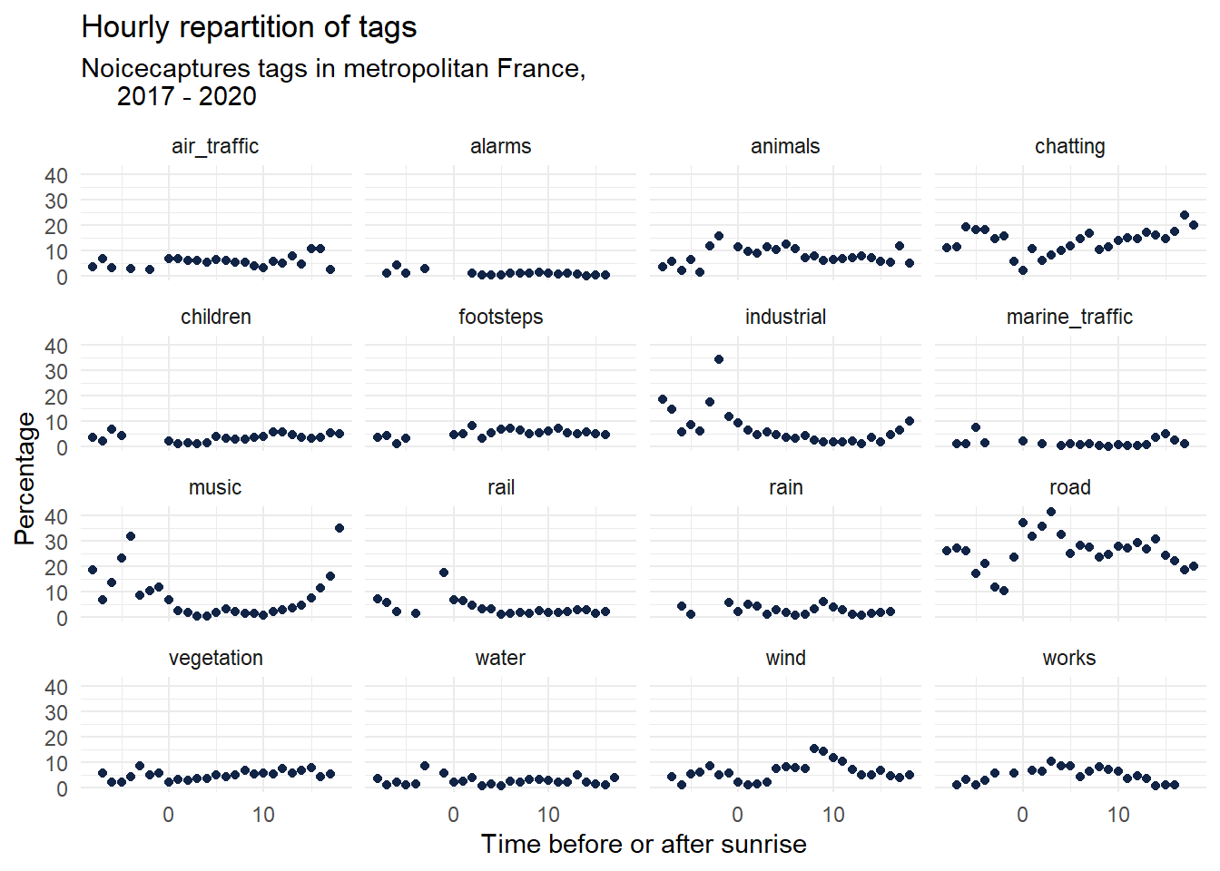

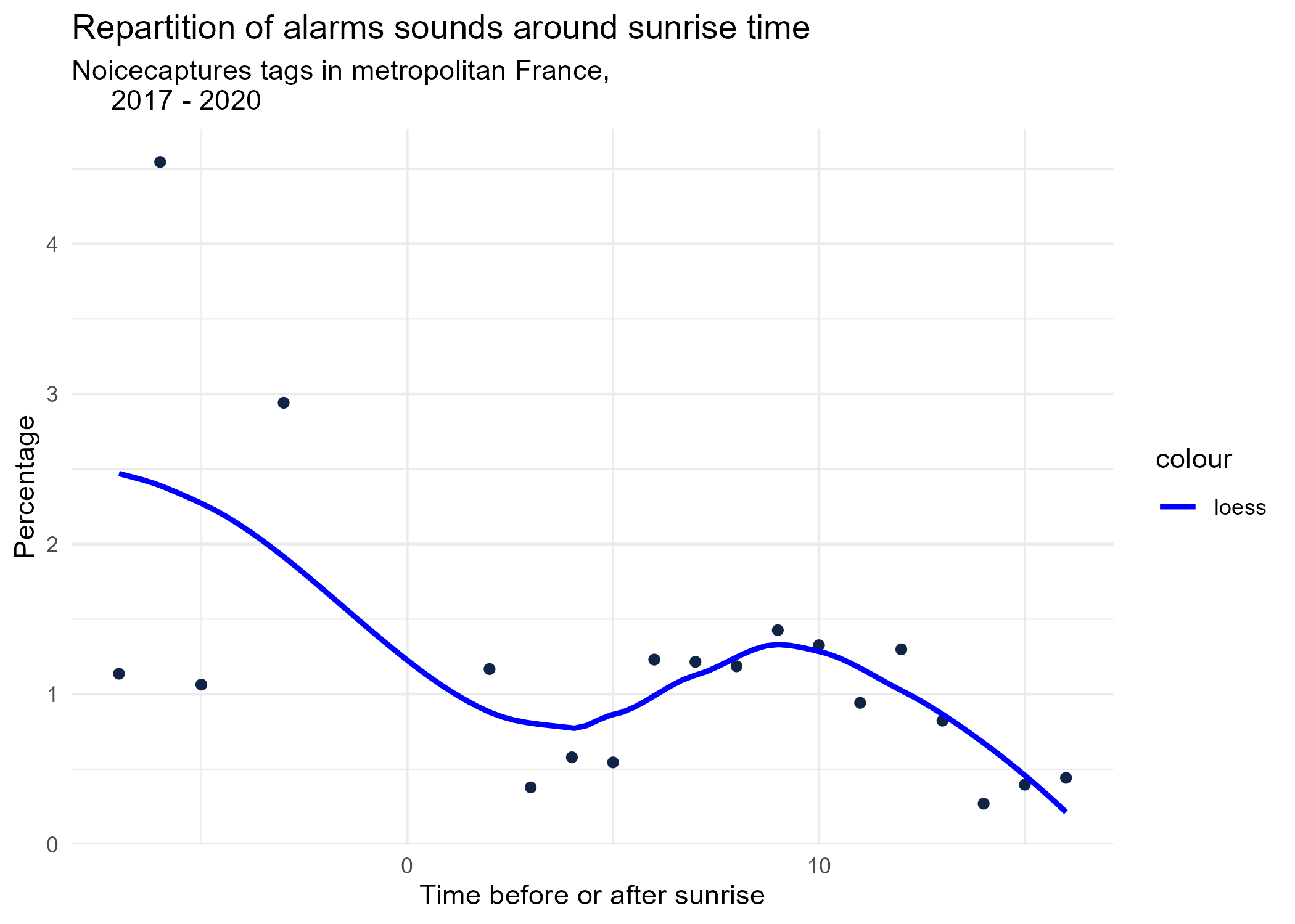
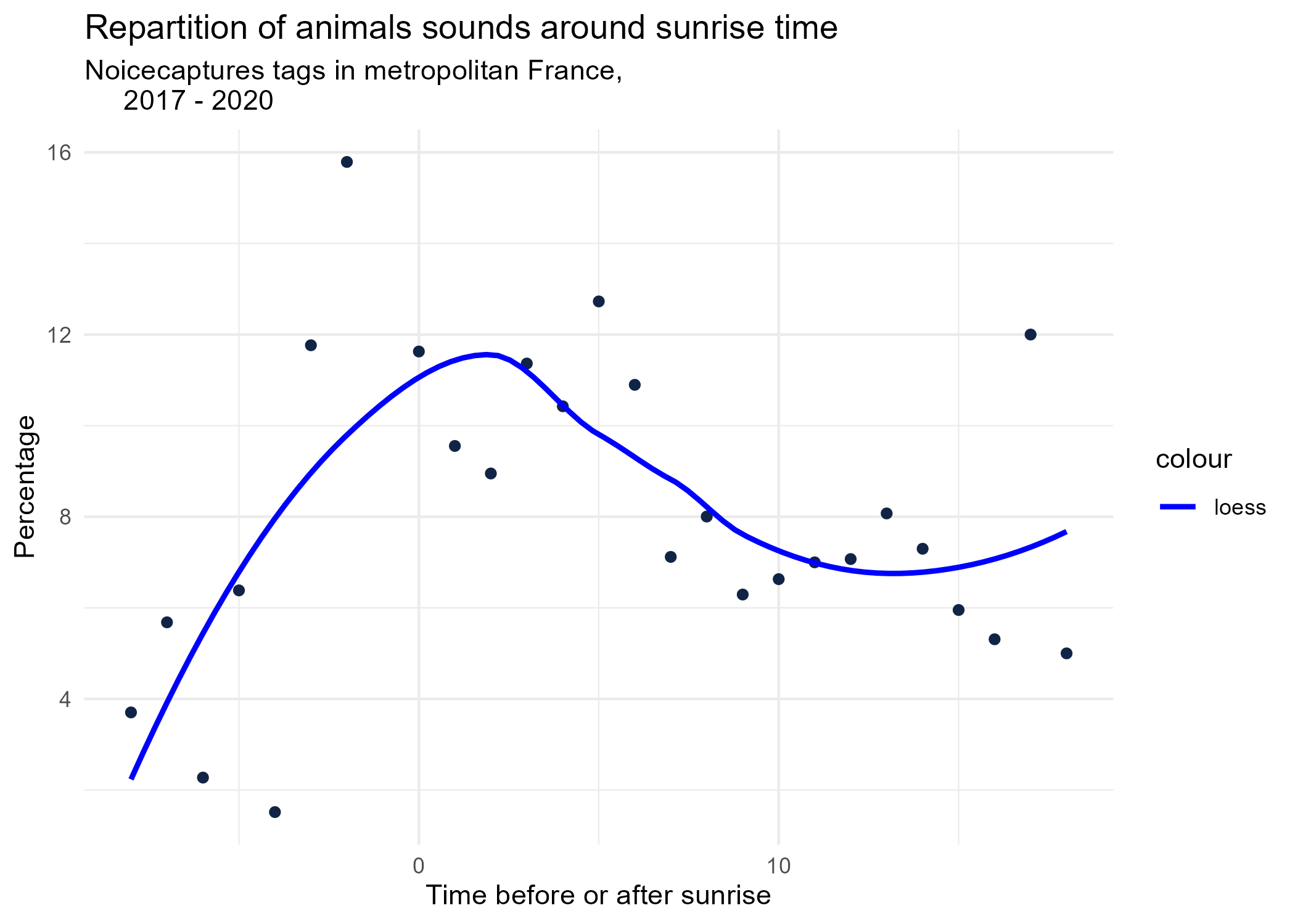
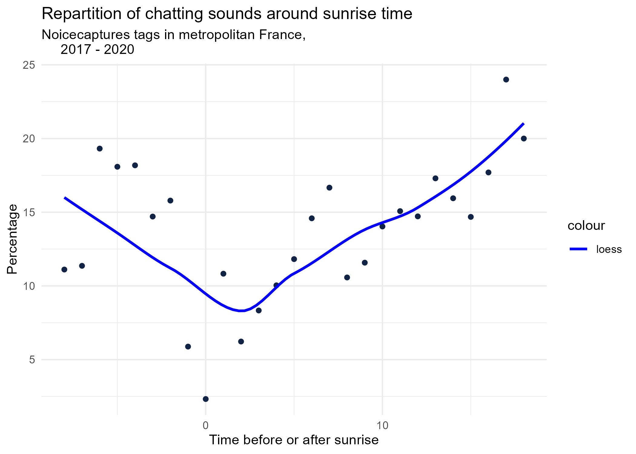
sunrise_graphs <- function(tag) {
  
  title <- paste("Repartition of",tag,"sounds around sunrise time")
  ggplot(time_after_sunrise_repartition %>% dplyr::filter(tag_name == tag)) +
   aes(x = time_after_sunrise, y = percentage) +
   geom_point(shape = "circle", size = 1.5, colour = "#112446") +
   labs(
     x = "Time before or after sunrise",
     y = "Percentage",
     title = title,
     subtitle = "Noicecaptures tags in metropolitan France,
     2017 - 2020"
   ) +
   geom_smooth(method = "loess", se = FALSE, aes(colour="loess")) + # smooth curve test (see span parameter to fit more to the peak before sunrise)
  # geom_smooth(method = "lm", formula = y ~ poly(x, 3), se = FALSE, aes(colour="Polynomial")) +
  scale_colour_manual(values=c("blue", "red"))+
   theme_minimal()
  
  # save graphs
  ggsave(paste0("plots/",gsub(" ", "_",title),".png")) 
}

# Render graphs
graphs <- purrr::map(unique(seasonal_occurences$tag_name), sunrise_graphs)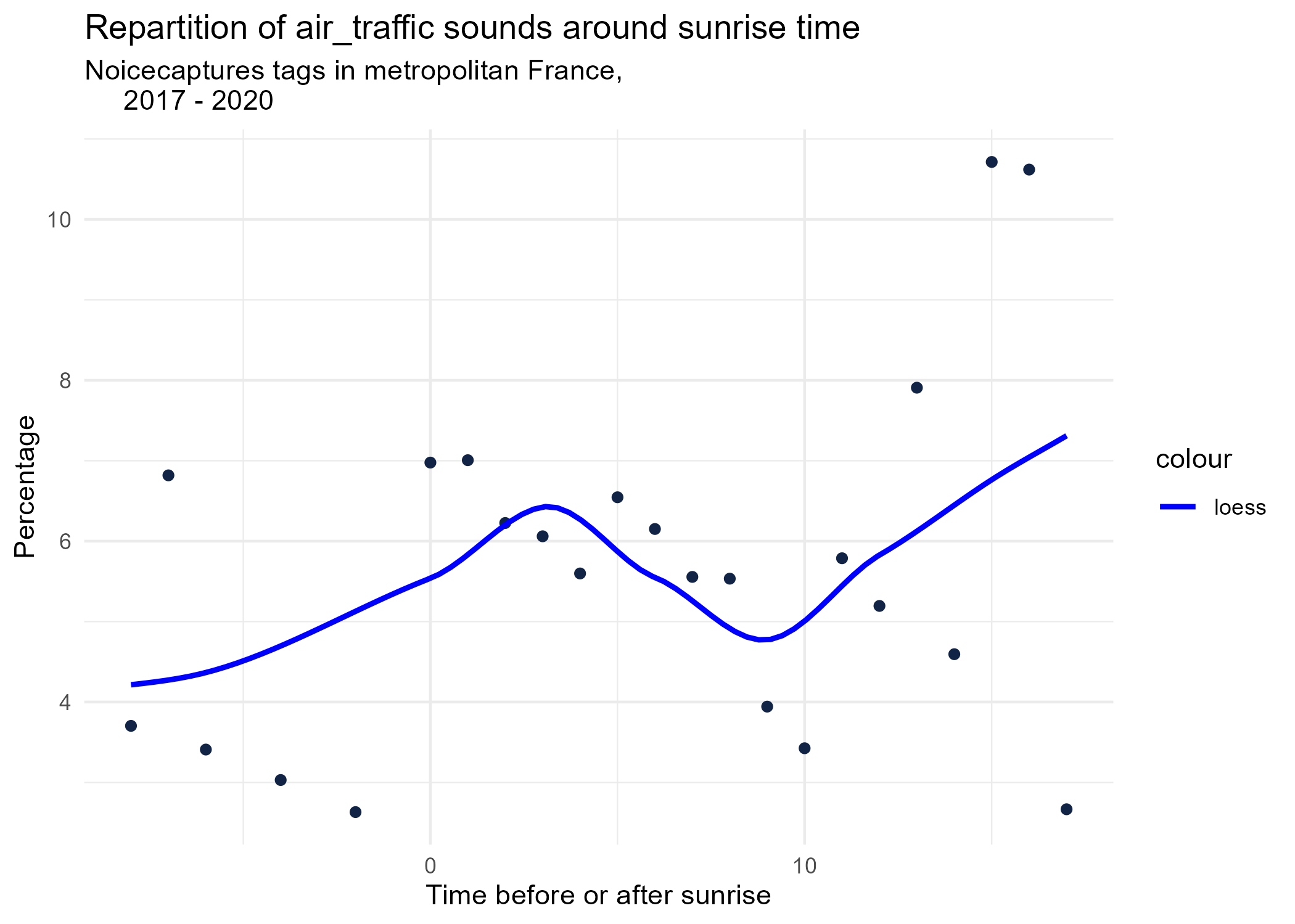

5 Monthly repartition

monthly_occurences <- all_info %>% dplyr::mutate(local_month = lubridate::month( # extract hour
    lubridate::with_tz( # convert to local time
      lubridate::ymd_hms(record_utc, tz = "UTC"), # convert text to date
      "Europe/Paris"))) %>%
  dplyr::group_by(tag_name, local_month, season) %>% 
  dplyr::count(name = "occurences")

tags_monthly_repartition <- monthly_occurences %>%  left_join(
    monthly_occurences %>% dplyr::group_by(local_month) %>% dplyr::summarise(total = sum(occurences)),
    by = "local_month") %>% 
  mutate(percentage = occurences * 100 / total)

data_breaks <- data.frame(start = c(0, 3, 6, 9),  # Create data with breaks
                          end = c(3, 6, 9, 12),
                          Seasons = factor(c("Winter", "Spring", "Summer", "Autumn"), 
                                          levels = c("Winter", "Spring", "Summer", "Autumn"),
                          labels = c("Winter", "Spring", "Summer", "Autumn")))
data_breaks                                       # Print data with breaks

##   start end Seasons
## 1     0   3  Winter
## 2     3   6  Spring
## 3     6   9  Summer
## 4     9  12  Autumn

ggplot() +
  # Add background colors to plot
  geom_rect(data = data_breaks,
            aes(xmin = start,
                xmax = end,
                ymin = - Inf,
                ymax = Inf,
                fill = Seasons),
            alpha = 0.25) +
  scale_fill_manual(values = c("Winter" = "white",
                               "Spring" = "green",
                               "Summer" = "yellow",
                               "Autumn" = "brown"
                               )) +
  geom_point(data = tags_monthly_repartition, aes(x = local_month, y = percentage),
             shape = "circle", size = 1.5, colour = "#112446") +
  labs(
    x = "Month",
    y = "Percentage",
    title = "Monthly repartition of tags",
    subtitle = "Noicecaptures tags in metropolitan France,
    2017 - 2020"
  ) +
  theme_minimal() +
  scale_x_continuous(breaks = scales::pretty_breaks(), labels=c("Jan","Feb","Apr","Jun", "Aug", "Oct", "Dec", "null"), limits = c(1,12))+
  facet_wrap(vars(tag_name))

## Warning: Removed 16 rows containing missing values (geom_rect).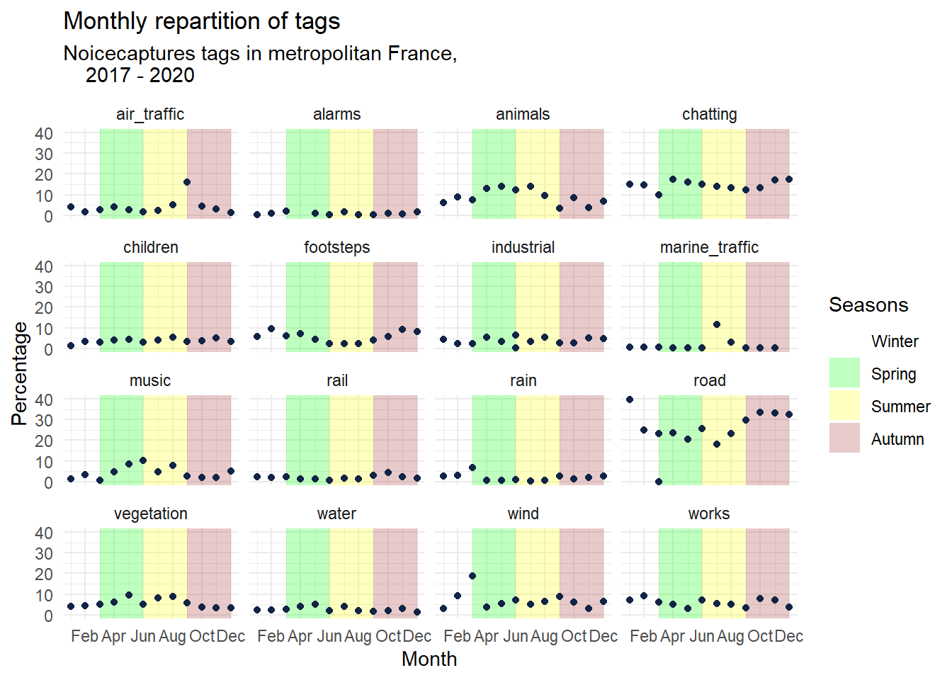

## Warning: Removed 16 rows containing missing values (geom_rect).

6 Packages citations

citation("tidyverse")

## 
##   Wickham et al., (2019). Welcome to the tidyverse. Journal of Open
##   Source Software, 4(43), 1686, https://doi.org/10.21105/joss.01686
## 
## A BibTeX entry for LaTeX users is
## 
##   @Article{,
##     title = {Welcome to the {tidyverse}},
##     author = {Hadley Wickham and Mara Averick and Jennifer Bryan and Winston Chang and Lucy D'Agostino McGowan and Romain François and Garrett Grolemund and Alex Hayes and Lionel Henry and Jim Hester and Max Kuhn and Thomas Lin Pedersen and Evan Miller and Stephan Milton Bache and Kirill Müller and Jeroen Ooms and David Robinson and Dana Paige Seidel and Vitalie Spinu and Kohske Takahashi and Davis Vaughan and Claus Wilke and Kara Woo and Hiroaki Yutani},
##     year = {2019},
##     journal = {Journal of Open Source Software},
##     volume = {4},
##     number = {43},
##     pages = {1686},
##     doi = {10.21105/joss.01686},
##   }

citation("sf")

## 
## To cite package sf in publications, please use:
## 
##   Pebesma, E., 2018. Simple Features for R: Standardized Support for
##   Spatial Vector Data. The R Journal 10 (1), 439-446,
##   https://doi.org/10.32614/RJ-2018-009
## 
## A BibTeX entry for LaTeX users is
## 
##   @Article{,
##     author = {Edzer Pebesma},
##     title = {{Simple Features for R: Standardized Support for Spatial Vector Data}},
##     year = {2018},
##     journal = {{The R Journal}},
##     doi = {10.32614/RJ-2018-009},
##     url = {https://doi.org/10.32614/RJ-2018-009},
##     pages = {439--446},
##     volume = {10},
##     number = {1},
##   }

citation("hydroTSM")

## 
## To cite hydroTSM in publications use:
## 
##   Mauricio Zambrano-Bigiarini. (2020) hydroTSM: Time Series Management,
##   Analysis and Interpolation for Hydrological ModellingR package
##   version 0.6-0. URL https://github.com/hzambran/hydroTSM.
##   DOI:10.5281/zenodo.839864.
## 
## A BibTeX entry for LaTeX users is
## 
##   @Manual{,
##     title = {hydroTSM: Time Series Management, Analysis and Interpolation for Hydrological Modelling},
##     author = {{Mauricio Zambrano-Bigiarini}},
##     year = {2020},
##     note = {R package version 0.6-0 . doi: https://doi.org/10.5281/zenodo.83964},
##     url = {https://github.com/hzambran/hydroTSM},
##   }
## 
## I have invested an important amount of time and effort in creating
## hydroTSM, please cite it if you use it !

citation("suncalc")

## 
## To cite package 'suncalc' in publications use:
## 
##   Benoit Thieurmel and Achraf Elmarhraoui (2019). suncalc: Compute Sun
##   Position, Sunlight Phases, Moon Position and Lunar Phase. R package
##   version 0.5.0. https://CRAN.R-project.org/package=suncalc
## 
## A BibTeX entry for LaTeX users is
## 
##   @Manual{,
##     title = {suncalc: Compute Sun Position, Sunlight Phases, Moon Position and Lunar
## Phase},
##     author = {Benoit Thieurmel and Achraf Elmarhraoui},
##     year = {2019},
##     note = {R package version 0.5.0},
##     url = {https://CRAN.R-project.org/package=suncalc},
##   }

7 Reproductibility

7.1 Data sources

Most of the treatment has been made within the PostGIS database. The scripts folder contains several scripts to execute to prepare the dataset.

7.2 Session informations

## R version 4.1.1 (2021-08-10)
## Platform: x86_64-w64-mingw32/x64 (64-bit)
## Running under: Windows 10 x64 (build 19044)
## 
## Locale:
##   LC_COLLATE=French_France.1252  LC_CTYPE=French_France.1252   
##   LC_MONETARY=French_France.1252 LC_NUMERIC=C                  
##   LC_TIME=French_France.1252    
## 
## Package version:
##   DBI_1.1.1         dplyr_1.0.9       ggplot2_3.3.5     hydroTSM_0.6-0   
##   lubridate_1.8.0   purrr_0.3.4       RPostgreSQL_0.7-3 scales_1.1.1     
##   sf_1.0-3          suncalc_0.5.0     xfun_0.30         xts_0.12.1       
##   zoo_1.8-9

7.3 Database information

# print software versions
pg_version  <- xfun::cache_rds({
  RPostgreSQL::dbGetQuery(con,statement = paste("SELECT version();")) # should return PostgreSQL 10.15 or higher
},rerun = params$database)
print(pg_version)

##                                                                                                                                version
## 1 PostgreSQL 10.21 (Ubuntu 10.21-0ubuntu0.18.04.1) on x86_64-pc-linux-gnu, compiled by gcc (Ubuntu 7.5.0-3ubuntu1~18.04) 7.5.0, 64-bit

postgis_version  <- xfun::cache_rds({
  RPostgreSQL::dbGetQuery(con,statement = paste("SELECT postgis_full_version();")) # should return PostGIS 2.5 or higher
},rerun = params$database)
print(postgis_version)

##                                                                                                                                                                                            postgis_full_version
## 1 POSTGIS="2.5.5" [EXTENSION] PGSQL="100" GEOS="3.7.1-CAPI-1.11.1 27a5e771" PROJ="Rel. 4.9.3, 15 August 2016" GDAL="GDAL 2.4.2, released 2019/06/28" LIBXML="2.9.4" LIBJSON="0.12.1" LIBPROTOBUF="1.2.1" RASTER

# close connection
RPostgreSQL::dbDisconnect(con)

Nicolas Roelandt

Pierre Aumond

Ludovic Moisan

2022-06-29