Dynamic Tutorial - GUI

Many publications have emerged showcasing the use of NoiseModelling to create dynamic maps (see scientific production).

If you’d like to achieve similar results but you feel a bit lost, this tutorial is here to help you navigate through the process.

There are three main approaches to creating dynamic maps using NoiseModelling:

A road network with a single traffic flow You have a road network and a single traffic flow associated with a specific time period (e.g., 24h). You want to compute dynamic indicators such as L10, L90, or the number of events exceeding a threshold or to get time series for the same time period.
A road network with traffic flows at regular intervals You have a road network and traffic flow data available at regular intervals (e.g., hourly or every 15 minutes), and you want to generate a dynamic noise map every 15 min.
A road network with associated spatio-temporal data of moving sources You have spatio-temporal information about vehicles moving around a network (e.g., from traffic simulations such as Simuvya or SUMO; or from trajectories of drones). You want to compute time-series data at each receiver corresponding to the passage of these sources.

A Word of Caution

Caution : In all these cases, we assume that the sound attenuation between the source and receiver remains constant throughout the calculation. This is a strong approximation, and there are ways to account for variations, but this tutorial will not cover such specific cases.

Dynamic mapping has its subtleties, and it’s important to be aware of them to avoid errors. We recommend referring to the following documents for a better understanding of these concepts:

Can, A., & Aumond, P. (2018). Estimation of road traffic noise emissions: The influence of speed and acceleration. Transportation Research Part D: Transport and Environment, 58, 155-171.
Gozalo, G. R., Aumond, P., & Can, A. (2020). Variability in sound power levels: Implications for static and dynamic traffic models. Transportation Research Part D: Transport and Environment, 84, 102339.
Le Bescond, V., Can, A., Aumond, P., & Gastineau, P. (2021). Open-source modeling chain for the dynamic assessment of road traffic noise exposure. Transportation Research Part D: Transport and Environment, 94, 102793.

Assumptions are freely made, specific formats are expected, and so on. To understand the required data formats and check the expected structure of the input tables, please refer also to the example input tables and spatial layers!

Case 1: A Road Network with a Single Traffic Flow

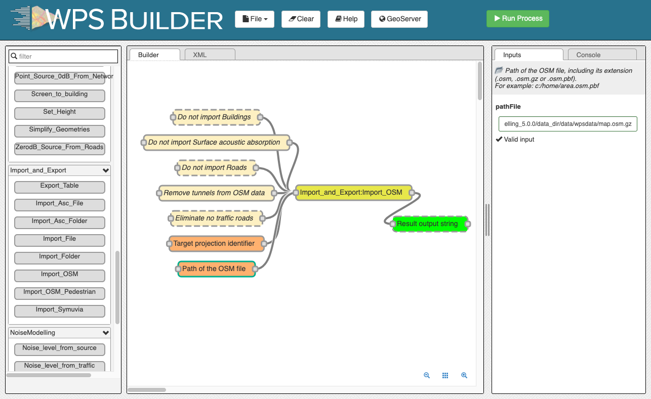
Import the road network (with arbitrary traffic flows) and buildings from an OSM file

Use Import_OSM WPS block

Path of the osm file: Enter the path of the provided Open Street map file (can be relative to NoiseModelling): data_dir/data/wpsdata/map.osm.gz
Target projection identifier: Enter the official France projection for this tutorial files 2154
Remove tunnels: Check it
Do not import surface: Check it as we will not use this output

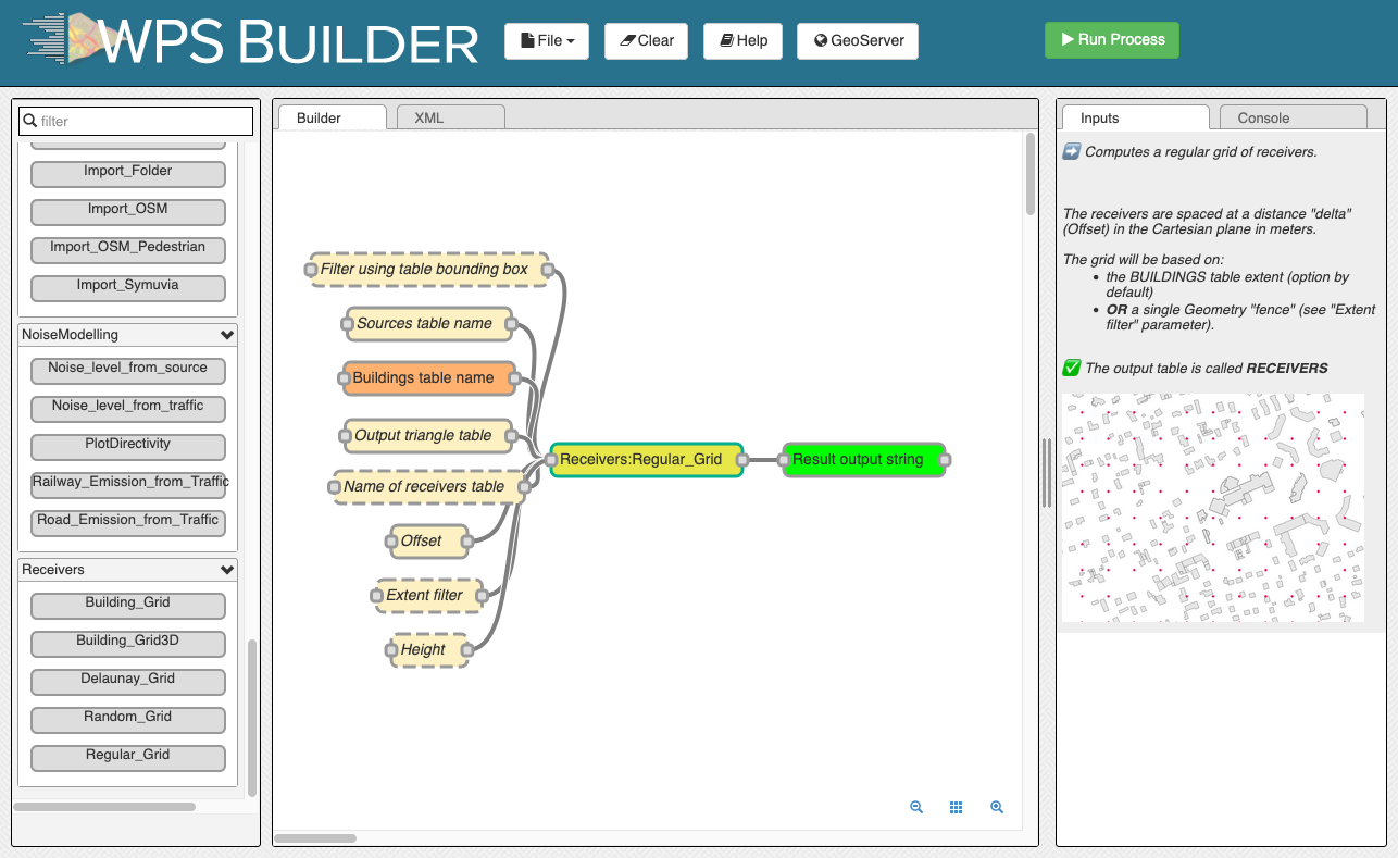
Create a receiver grid using 25 meters step in a grid pattern

Use Regular_Grid WPS block

Table bounding box name: Enter ROADS The receivers will use the envelope of the ROADS table.
Offset: Enter 15 for 15 meters distance
Output triangle table: Check it in order to be able to generate the iso contours
height: Enter 1.5

Convert traffic to dynamic traffic flow

From the network with traffic flow to individual trajectories with associated Lw

The Probabilistic method, this method place randomly the vehicles on the network according to the traffic flow
The Poisson method place the vehicles on the network according to the traffic flow following a poisson law,

it keeps a coherence in the time series of the noise level

Use the Dynamic:Flow_2_Noisy_Vehicles WPS block:

Method: Enter TNP Use the Poisson method
Roads table name: Enter ROADS
timestep: Enter 1
duration: Enter 60
gridStep: Enter 10

Compute noise level at receivers points for each receiver-period

Use the NoiseModelling:Noise_level_from_source WPS block

Buildings table name: Enter BUILDINGS
Source geometry table name: Enter SOURCES_GEOM Contain only the geometries of the sources (points)
Source emission table name: Enter SOURCES_EMISSION Contain for each source index and period the noise emission
Receivers table name: Enter RECEIVERS
Max Error (dB): Enter 3 Will skip further sources, reduce the computation time for this tutorial
Maximum source receiver distance: Enter 800
Diffraction on horizontal edges: Check it
Order of reflexion: Enter 0

Compute noise indicators

This step is optional, it compute the LA10, LA50 and LA90 at each receiver from the table RECEIVERS_LEVEL

Use the Acoustic_Tools:DynamicIndicators wps block

tableName: Enter RECEIVERS_LEVEL
columnName: Enter LAEQ

Compute iso-surfaces for each time period

Generate a dynamic iso-contour map for each time period based on the LAEQ of the receivers.

Use the Acoustic_Tools:Create_Isosurface wps block

Sound levels table: Enter RECEIVERS_LEVEL
Smooth coefficient: Enter 0

Export Map to QGis

Using Export_Table block export the following tables as files in any folder.

CONTOURING_NOISE_MAP
BUILDINGS
ROADS

Configure QGis to display time dependant map

Load the 3 files in QGIS. Contouring_noise_map must be ordered as the last layer (rendered in the bottom)

Load the style for contouring noise map:

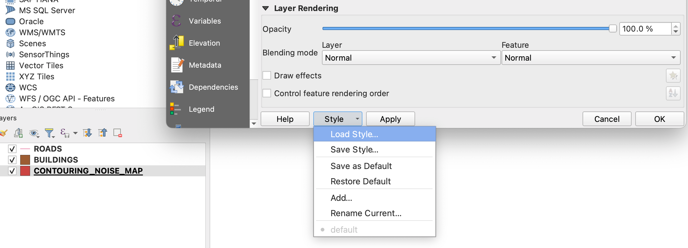
Load the style located in the NoiseModelling folder Docs/styles/style_beate_tomio.sld

In QGis in time window paste the following formulae:

datetime_from_epoch(to_real("PERIOD")*1000+1739869220000) datetime_from_epoch(to_real("PERIOD")*1000+1739869221000)

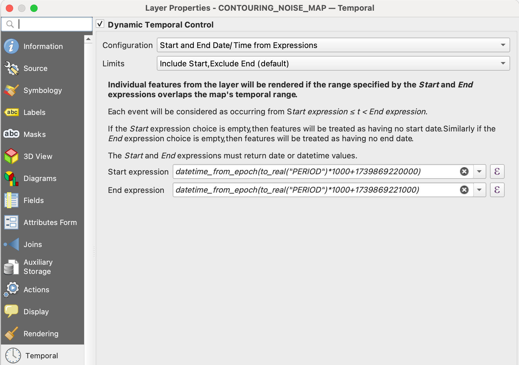
Epoch is in millisecond, so we multiply by 1000 and add any base epoch time. The step end 1000 milliseconds after the start period.

With the navigation bar of QGis you can select the period to display.

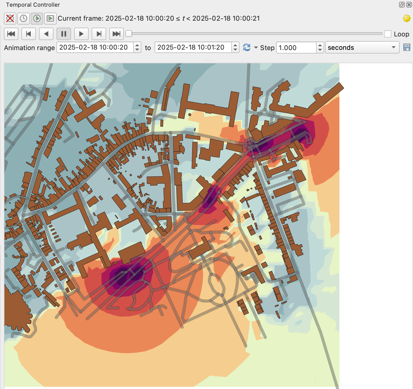
Case 2: A Road Network with Traffic Flows at Regular Intervals

This case is similar to the MATSim use case (here), but this tutorial generalizes the approach to fit other datasets.

This sample dataset used in this example was kindly provided by Valentin Lebescond from Université Gustave Eiffel.

Import Buildings for your study area

Use Import File WPS block

Path of the input File: Enter the path of building (can be relative to NoiseModelling): data_dir/data/wpsdata/Dynamic/Z_EXPORT_TEST_BUILDINGS.geojson
Projection identifier: Enter SRID 2154
Output table name: Enter buildings

Import the road network

Use Import File WPS block

Path of the input File: Enter the path of building (can be relative to NoiseModelling): data_dir/data/wpsdata/Dynamic/Z_EXPORT_TEST_TRAFFIC.geojson
Projection identifier: Enter SRID 2154
Output table name: Enter roads

Create a receiver grid using 25 meters step in a grid pattern

Use Regular_Grid WPS block

Table bounding box name: Enter ROADS The receivers will use the envelope of the ROADS table.
Offset: Enter 25 for 25 meters distance
height: Enter 1.5

Split geometry and traffic periods

In the table ROADS, the traffic information is given for each period in the TIME column.

The following WPS block aggregate roads by the geometry and place the associated pair IDSOURCE/PERIOD with the corresponding road traffic into the SOURCES_EMISSION table.

Use the block Dynamic::Split_Sources_Period :

Source table name: Enter ROADS
Source index field name: Enter LINK_ID
Source period field name: Enter TIME. The field time will be renamed to PERIOD.

Two output table is created SOURCES_GEOM and SOURCES_EMISSION

Compute noise level at receivers points for each receiver-period

Use the NoiseModelling:Noise_level_from_source WPS block

Buildings table name: Enter BUILDINGS
Source geometry table name: Enter SOURCES_GEOM Contain only the geometries of the sources (points)
Source emission table name: Enter SOURCES_EMISSION Contain for each source index and period the noise emission
Receivers table name: Enter RECEIVERS
Diffraction on horizontal edges: Check it
Order of reflexion: Enter 0

Compute noise indicators

This step is optional, it compute the LA10, LA50 and LA90 at each receiver from the table LT_GEOM

Use the Acoustic_Tools:DynamicIndicators wps block

tableName: Enter RECEIVERS_LEVEL
columnName: Enter LAEQ

The result table LT_GEOM can be displayed into QGis, if you filter by PERIOD.

Case 3: Spatio-Temporal Data of Moving Sources

This sample dataset was kindly provided by Sacha Baclet from KTH (0000-0003-2114-8680).

Import Buildings for your study area

Use Import File WPS block

Path of the input File: Enter the path of building (can be relative to NoiseModelling): data_dir/data/wpsdata/Dynamic/buildings_nm_ready_pop_heights.shp
Projection identifier: Enter SRID 32635
Output table name: Enter buildings

Import the receivers (or generate your set of receivers using Regular_Grid script for example)

Use Import File WPS block

Path of the input File: Enter the path of building (can be relative to NoiseModelling): data_dir/data/wpsdata/Dynamic/receivers_python_method0_50m_pop.shp
Projection identifier: Enter SRID 32635
Output table name: Enter receivers
height: Enter 1.5

Import the road network

Use Import File WPS block

Path of the input File: Enter data_dir/data/wpsdata/Dynamic/network_tartu_32635_.geojson
Projection identifier: Enter SRID 32635
Output table name: Enter network_tartu

Add primary key column to the road network (Optional)

Use Add_Primary_Key WPS block

Name of the column: Enter PK
Name of the table: Enter SRID network_tartu

Import the vehicles trajectories

Use Import File WPS block

Path of the input File: Enter data_dir/data/wpsdata/Dynamic/SUMO.geojson
Projection identifier: Enter SRID 32635
Output table name: Enter vehicle

Create point sources from the network every 10 meters

This point source will be used to compute the noise attenuation level from them to each receiver. The created table will be named SOURCES_GEOM.

Use Point_Source_From_Network WPS block

Input table name: Enter network_tartu
gridStep: Enter SRID 10

Create a table with the noise level from the vehicles and snap the vehicles to the point sources

Use Ind_Vehicles_2_Noisy_Vehicles WPS block

Source geometry table: Enter SOURCES_GEOM
Individual Vehicles table: Enter vehicle
Snap distance: Enter 30 This is the maximal distance (m) to reattach individual vehicles position to the source points
Vehicles table format: Enter SUMO

Compute noise attenuation for each receiver-source pairs

Unlike the previous tutorial we will use an alternative approach here by storing the attenuation between all sources and receivers first. The applying later this attenuation to the emission level for each period.

Use the NoiseModelling:Noise_level_from_source WPS block

Buildings table name: Enter BUILDINGS
Source geometry table name: Enter SOURCES_GEOM Contain only the geometries of the sources (points)
Receivers table name: Enter RECEIVERS
Maximum source receiver distance: Enter 300
Diffraction on horizontal edges: Check it
Order of reflexion: Enter 0
Separate receiver level by source identifier: Check it to have the SOURCEID column on the output

Apply attenuation on emission levels

Compute the noise level from the moving vehicles to the receivers. The output table is called here LT_GEOM and contains the time series of the noise level at each receiver.

Use the Dynamic:Noise_From_Attenuation_Matrix WPS block

LW(PERIOD): Enter SOURCES_EMISSION
Attenuation Matrix Table name: Enter RECEIVERS_LEVEL
outputTable Matrix Table name: Enter LT_GEOM

Compute noise indicators

This step is optional, it compute the LA10, LA50 and LA90 at each receiver from the table LT_GEOM

Use the Acoustic_Tools:DynamicIndicators wps block

tableName: Enter RECEIVERS_LEVEL
columnName: Enter LAEQ

The result table LT_GEOM can be displayed into QGis, if you filter by PERIOD.

Note

All this tutorial done with Groovy is written on this unit test source code: Github source