Noise Map from Point Source - GUI

In this tutorial, we are going to produce a noise map, based on a unique source point. The exercice will be made through NoiseModelling with Graphic User Interface (GUI).

To make it more simple, we will use the data used in the Get Started - GUI tutorial.

This tutorial is divided in 5 steps:

1. Create the source point

2. Import data in NoiseModelling

3. Generate the noise map

4. Play with options

5. Take into account directivity

Step 1: Create the source point

To create the source point, we will use the free and opensource GIS software QGIS.

Note

For those who are new to GIS and want to get started with QGIS, we advise you to follow this tutorial as a start.

Load data into QGIS

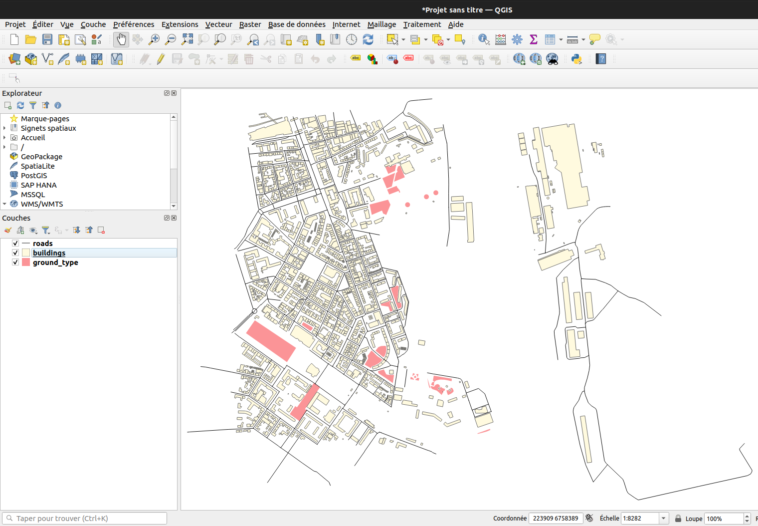
Once installed, launch QGIS and load the three buildings.shp, roads.shp and ground_type.shp files (that are in the folder ../NoiseModelling_5.0.0/data_dir/data/wpsdata/). To do so, you can just drag & drop these files into the Layers menu (bottom left of the user interface). Or you can also select them thanks to the dedicated panel opened via the Layer / Add a layer / Add a vectorial layer... / menu (or use Ctrl+Maj+V shortcut)

You should see your input data in the map as below:

Initialize the source point layer

In QGIS, we will create a new empty layer called Point_Source in which we will add the source point.

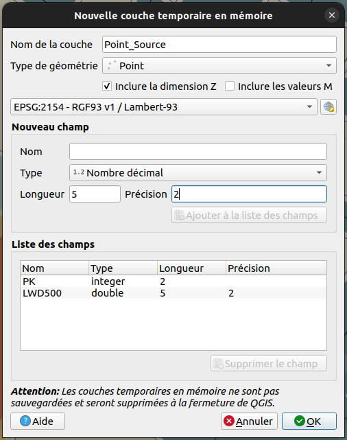
To do so, click on the Layer / Create Layer / New Temporary Scratch Layer... / menu. In the opened dialog, fill the detailed information below :

• File name : Point_Source

• Geometry type : choose Point in the dropdown list

• Include Z dimension : check the box. This way the created point will be defined with X, Y and Z coordinates

• In the projection system dropdown list, choose a metric system. Here we will choose the one used for the buildings, roads and ground_type layers, that are in metropolitan France : Lambert 93 system = EPSG:2154 (if the system is not present in the dropdown list, use the Globe icon on the right to find it)

In the New field part, fill the information below:

• Name : PK . Unique id (Primary Key)

• Type : Integer

• Length : 2

Once done, click on Add to Fields List. Then redo this step with the following informations:

• Name : HZD500 . Source noise level during the day (D) at a frequency of 500 Hz

• Type : Decimal number

• Length : 5

• Precision : 2

You should have something like this

Once done, click on OK button. The new layer Point_Source should appear in your Layers panel.

Add a new source point

Now we have an empty layer. It’s time to feed it with a point geometry.

By default, the new temporary layer is already turned into edtion mode. If not, you can activate it thanks to these two options:

• In the Layers panel, select the Point_Source layer and make a right-click. Choose Toggle Editing

• or you can click on the “Yellow pencil” icon in the toolbar

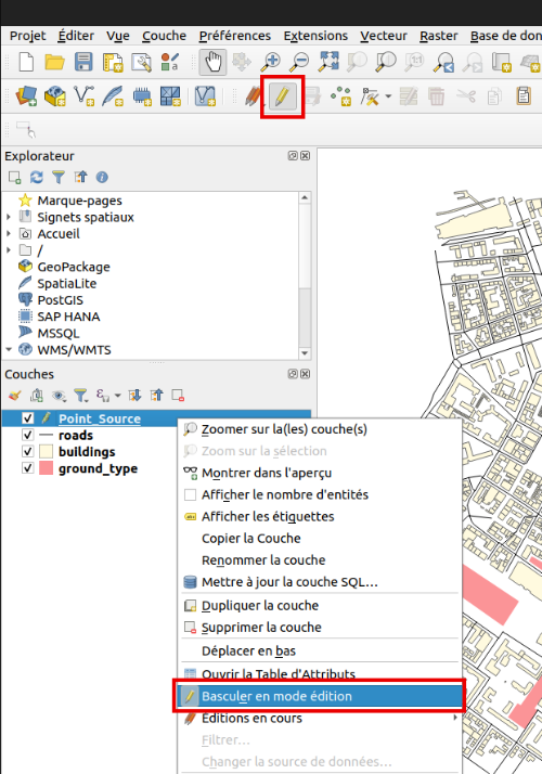
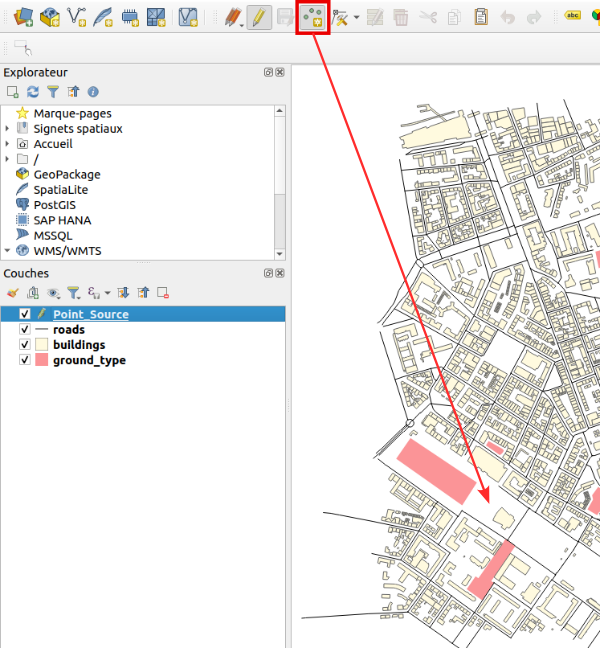
Now we can add a new point, by clicking on the dedicated icon (see illustration below) and then by clicking somewhere in the map.

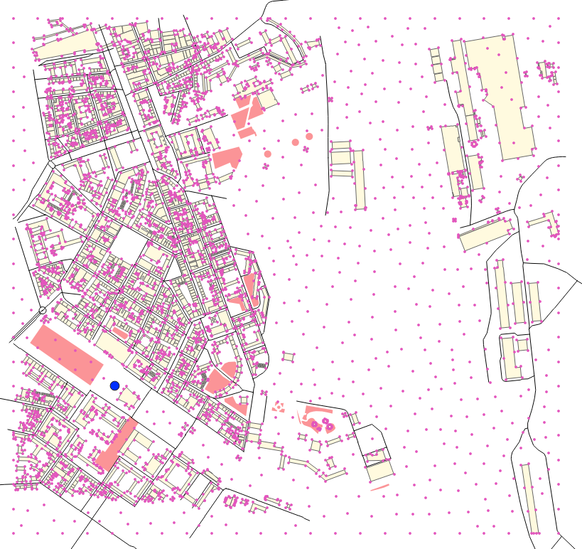
To have an interesting resulting noise map, choose to place your source point next to buildings.

Click on the map where you want to create the source point. Once clicked, a new dialog appears and you are invited to fill the following attributes:

• PK: 1

• HZD500 : 90

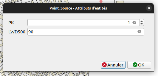
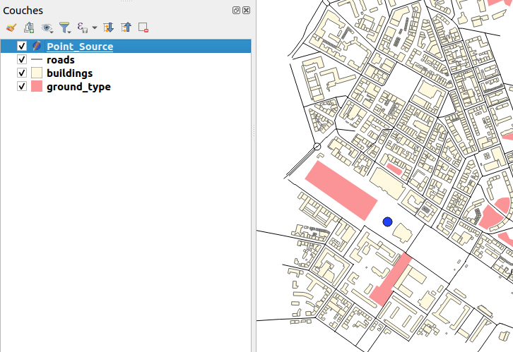
Once done, click on OK. The source point is now visible in the map (the blue point in the illustration below).

Now, we have to save this temporary layer into a flat file. To do so, just make a right-click on the layer name and choose the Make permanent option.

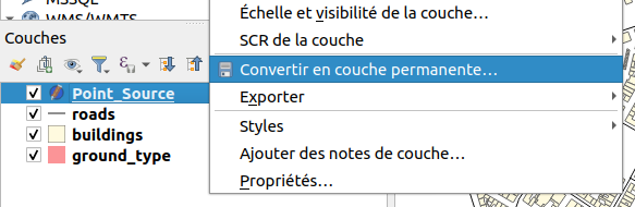
In the new dialog, select GeoJSON file format and then define the path and the name of your resulting .geojson file. Press OK when ready.

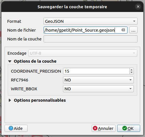
Your Point_Source.geojson file is now ready to be imported in NoiseModelling.

For your information, you can open .geojson files in most of text editor. If you do so with Point_Source.geojson, you will have something like this:

{
"type": "FeatureCollection",
"name": "Point_Source",
"crs": {"type": "name", "properties": { "name": "urn:ogc:def:crs:EPSG::2154" } },
"features": [{"type": "Feature", "properties": { "PK": 1, "HZD500": 90.0 },
              "geometry": {"type": "Point", "coordinates": [223771.0727, 6757583.2983, 0.0]}
             }]
}

Step 2: Import input data in NoiseModelling

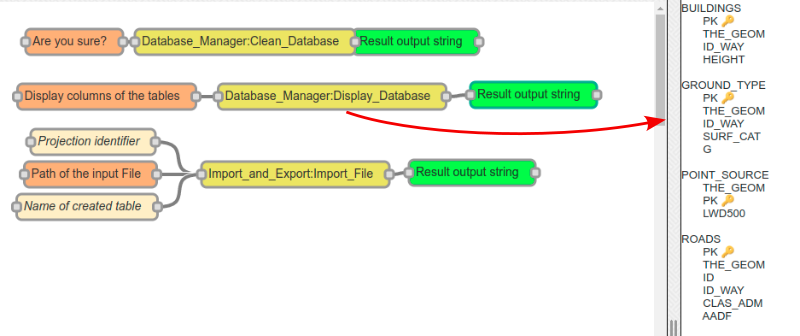
Once NoiseModelling is launched (see Step 2: Start NoiseModelling GUI in Get Started - GUI page), load the four BUILDINGS, ROADS and GROUND_TYPE, POINT_SOURCE layers (see Step 4: Load input files for more details).

If you use the Database_Manager:Display_Database WPS script, you should see your four tables like below:

Step 3: Generate the noise map

We are now ready to generate the noise map, based on a unique source point.

Create the receivers grid

Use the Receivers:Delaunay_Grid WPS script. Fill the two following mandatory parameters (in orange) and click on Run Process button:

• Source table name : POINT_SOURCE

• Buildings table name : BUILDINGS

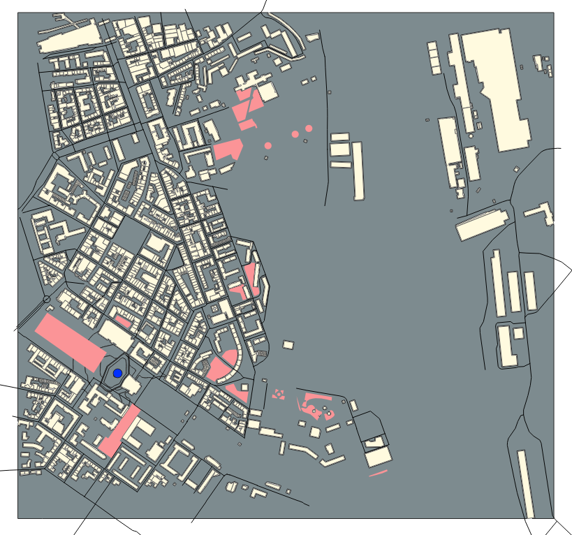
Once done, you should have two new tables : RECEIVERS (illustrated below with the purple small points) and TRIANGLES

Calculate noise levels

Use the NoiseModelling:Noise_level_from_source WPS script. Fill the three following mandatory parameters (in orange):

• Source table name : POINT_SOURCE

• Receivers table name : RECEIVERS

• Buildings table name : BUILDINGS

Once ready, click on Run Process button.

You should then have this message: Calculation Done ! RECEIVERS_LEVEL table(s) have been created.

Generate noise level isosurfaces

Use the Acoustic_Tools:Create_Isosurface WPS script. Fill the following mandatory parameter (in orange) and click on Run Process button:

• Sound levels table : RECEIVERS_LEVEL

You should have this message: Table CONTOURING_NOISE_MAP created

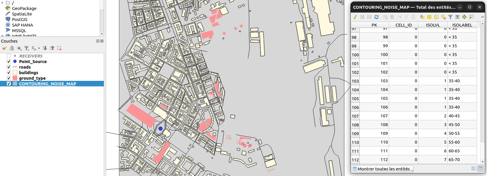
Now, you can export this table into a .shapefile, using the Import_and_Export:Export_Table WPS script.

You can then visualize this file into QGIS (just load the file as seen before). The resulting table (in grey) is illustred below

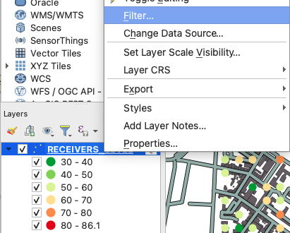
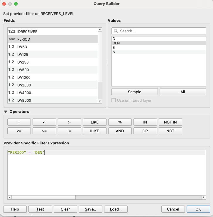
Filter the table according to a single period (ex. DEN):

Apply a color palette adapted to acoustics

In QGIS, since the isosurface table is not easy to read (everything is grey in our example), we will change the color palette to have colors depending on the noise levels. This information is present in the field ISOLVL in the attributes table. To open it, just select the layer CONTOURING_NOISE_MAP and press F6.

To adapt the colors, we will apply a cartographic style. This style:

• has been proposed by B. Tomio (Weninger) in “A Color Scheme for the Presentation of Sound Immission in Maps : Requirements and Principles for Design” (see publication and website)

• is provided (by NoiseModelling team) as a .sld (Style Layer Descriptor) file and can be downloaded here

Note

If you want to know more about noise map styles, you should read the “Noise Map Color Scheme” page.

Once downloaded, make a double click on the layer CONTOURING_NOISE_MAP. It will opens the property panel. Here, click on the Symbology tab. In the Style menu (at the bottom), choose Load style. Then in the opened dialog, click on the ... icon to search the style_beate_tomio.sld file. Once selected, click on Load style.

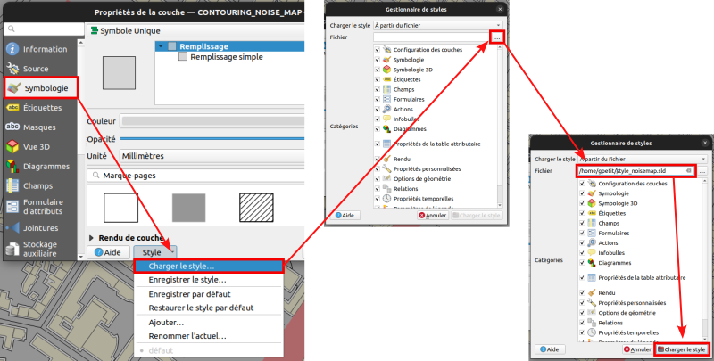
The style with its different colors is now displayed.

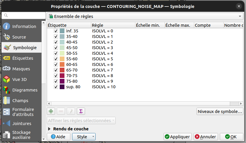
Press OK to apply and close the dialog. Your noise map is now well colorized and you can navigate into it to see the influence of buildings on noise levels.

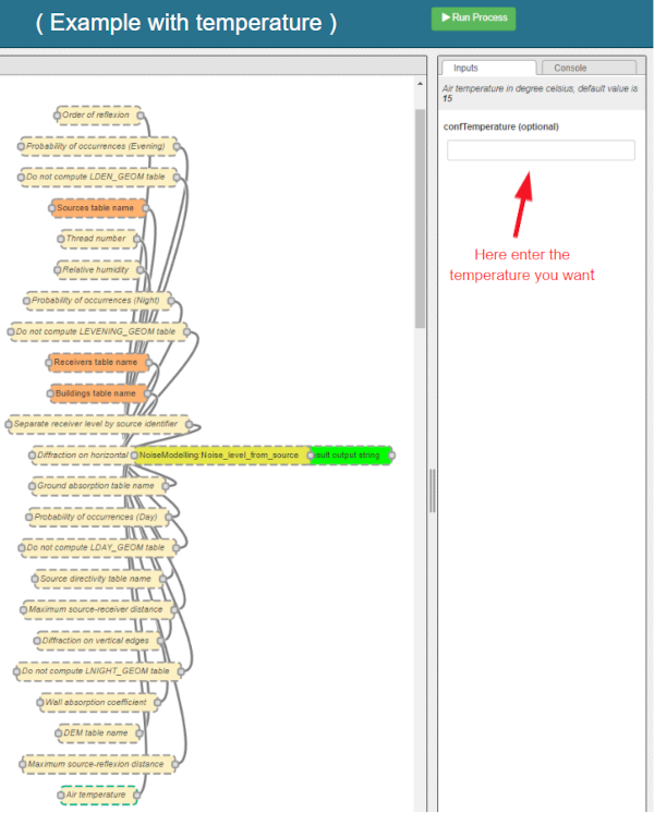
Step 4: Change the default parameters

To produce this noise map, we used, in most of WPS scripts, default parameters (e.g the height of the source, the number of reflections, the air temperature, …). You are prompted to redo some of the previous steps by changing some of the settings. You will then be able to visually see what impact they have on the final noise map.

Note

To change optionnal parameters (the yellow boxes) just select them and fill the needed informations in the right-side menu.

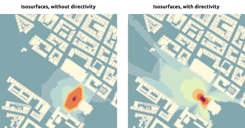
Step 5 (bonus): Change the directivity

In this bonus step, we will manage with the directivity. To do so, we will apply the following method:

1. Get directivity

2. Update the Source_Point table

3. Import needed data into NoiseModelling

4. Produce the noise map, taking into acount directivity parameters

Directivity

The directivity table aims at modeling a realistic directional noise source. To do so, we associate to each “Theta-Phi” pair an attenuation in dB.

• DIR_ID : identifier of the directivity sphere

• THETA : vertical angle in degrees, 0 (front), -90 (bottom), 90 (top), from -90 to 90

• PHI: horizontal angle in degrees, 0 (front) / 90 (right), from 0 to 360

• HZ500 : attenuation levels in dB for 500 Hz

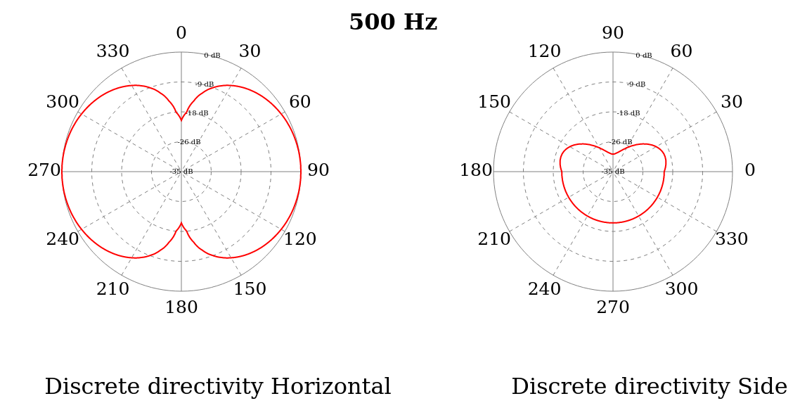
Each of the sound sources has its own directivity. For the exercise we will use the directivity of a train, which is provided in the file Directivity.csv and which you are invited to download.

Extract from the directivity table (Directivity.csv)

DIR_ID	THETA	PHI	HZ500
1	-90	0	-20
1	-85	0	-20
1	-80	0	-20
1	-75	0	-20
1	-70	0	-20
1	-65	0	-20
…	…	…	…

Below is an illustration generated from train directivity formula.

Update source point table

To play with directivity, we need to add 4 fields in the source point table:

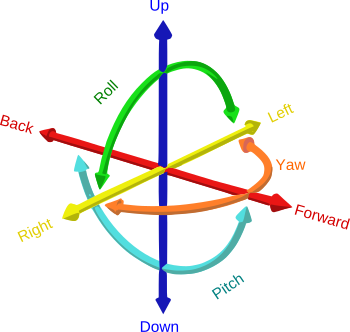
• Yaw

  • Name : YAW

  • Description : Source horizontal orientation in degrees. For points 0° North, 90° East. For lines 0° line direction, 90° right of the line direction.

  • Type : Decimal number

  • Length : 4

• Pitch

  • Name : PITCH

  • Description : Source vertical orientation in degrees. 0° front, 90° top, -90° bottom. (FLOAT).

  • Type : Decimal number

  • Length : 4

• Roll

  • Name : ROLL

  • Description : Source roll in degrees

  • Type : Decimal number

  • Length : 4

• Direction identififier

  • Name : DIR_ID

  • Description : Identifier of the directivity sphere from tableSourceDirectivity parameter or train directivity if not provided -> OMNIDIRECTIONAL(0), ROLLING(1), TRACTIONA(2), TRACTIONB(3), AERODYNAMICA(4), AERODYNAMICB(5), BRIDGE(6)

  • Type : Integer

  • Length : 2

Note

Source image: GregorDS, CC BY-SA 4.0, via Wikimedia Commons

In our example, we will update the Point_Source.geojson file to add these columns and to fill them with new information. To do so, just edit the file into a text editor and replace the following lines. Save it once done.

{ "PK": 1, "HZD500": 100.0}

by

{ "PK": 1, "HZD500": 100.0, "YAW": 45, "PITCH": 0, "ROLL": 0, "DIR_ID" : 1 }

Here we can see that the Yaw is setted to 45°. Pitch and Roll are equal to 0, and the directivity is defined as 1 and will refer to the directivy table (see below).

So your final .geojson file should look like this

{
"type": "FeatureCollection",
"name": "Point_Source",
"crs": {"type": "name", "properties": { "name": "urn:ogc:def:crs:EPSG::2154" } },
"features": [{"type": "Feature", "properties": { "PK": 1, "HZD500": 100.0, "YAW": 45, "PITCH": 0, "ROLL": 0, "DIR_ID" : 1 },
              "geometry": {"type": "Point", "coordinates": [223771.0727, 6757583.2983, 0.0]}
             }]
}

Import data

Now, in NoiseModelling we have to:

• Import the Directivy.csv file

• Reimport the Point_Source.geojson file in order to take into account the changes

• Import the dem.geojson file, which is placed here ./NoiseModelling_5.0.0/data_dir/data/wpsdata/dem.geojson. By taking into account the ground elevation, this file will help us to get better results.

To do so, just use the Import_and_Export:Import_Table WPS script.

Generate the Delaunay triangulation

Use the Receivers:Delaunay_Grid WPS script. Fill the following parameters and click on Run Process button:

• Sources table name : POINT_SOURCE

• Maximum Area : 60

• Buildings table name: BUILDINGS

• Height : 1.6

Compute noise level from source

Use the NoiseModelling:Noise_level_from_source WPS script. Fill the following parameters and click on Run Process button:

• Sources table name : POINT_SOURCE

• Buildings table name : BUILDINGS

• Receivers table name : RECEIVERS

• Ground absorption table name : GROUND_TYPE

• Source directivity table name : DIRECTIVITY

• Maximum source-receiver distance : 800

• DEM table name : DEM

Create isosurface

Use the Acoustic_Tools:Create_Isosurface WPS script. Fill the following parameters and click on Run Process button:

• Sound levels table : RECEIVERS_LEVEL

• Polygon smoothing coefficient : 0.4

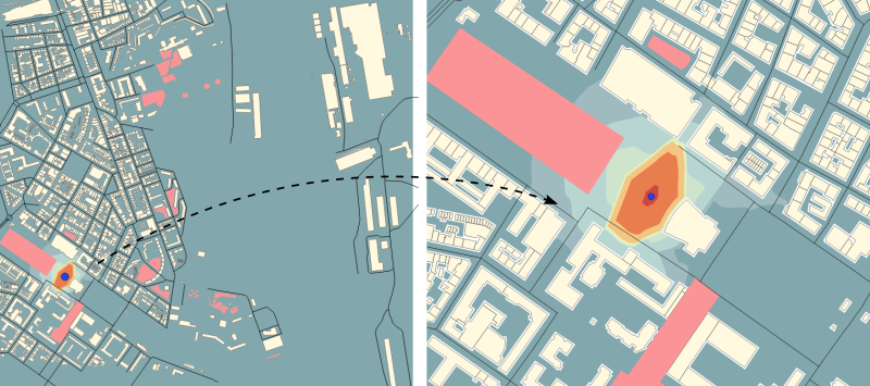
Export and visualize resulting tables

Use the Import_and_Export:Export_Table WPS script to export the CONTOURING_NOISE_MAP table into a shapefile called CONTOURING_NOISE_MAP_DIRECTIVITY.

Then, load CONTOURING_NOISE_MAP_DIRECTIVITY.shp into QGIS and filter the period to DEN. Apply the noisemap_style.sld style, and compare with CONTOURING_NOISE_MAP.shp produced in Step 3.