Data Assimilation

Introduction

Data assimilation is a technique that combines observations with a numerical model to improve the accuracy of forecasts or analyses. Applied to acoustics and noise maps, data assimilation makes it possible to integrate real noise measurements (e.g coming from sensors) into noise propagation models to produce more accurate and reliable noise maps.

In this tutorial, we will see how to model and simulate noise in Geneva 🇨🇭 using static (road network, buildings) and dynamic (traffic, temperature) data. The main objective is to combine measurements from sensors located in Geneva with acoustic simulations to identify traffic configurations that best match measurements.

Requirements

To play with this tutorial, you will need:

a working installation of NoiseModelling (NM) with at least version 5.0.1. If needed, get the last release on the official GitHub repository,
the tutorial’s datasets, stored in the folder .../NoiseModelling_5.0.1/data_dir/data/wpsdata/dataAssimilation/,
the dedicated WPS .groovy scripts, stored in the folder .../NoiseModelling_5.0.1/data_dir/scripts/wps/DataAssimilation/.

The data

In the the tutorial’s folder, you have the following data:

sensor measurement .csv files, stored in the devices_data/ folder (One file per sensor),

device_mapping_sf.geojson containing two columns : the point geometry (THE_GEOM) and a sensor’s unique identifier (DEVEUI`). This file is also provided in .csv format,

the OpenStreetMap (OSM) dataset of the studied area : geneva.osm.pbf.

Sensor measurements

Each .csv files in the folder devices_data/ contains environmental noise measurements recorded by individual sensors. The columns are:

deveui : Unique identifier of the sensor,
epoch : Time of measurement (Epoch format - Unix time, ex:1724567400),
Leq : Equivalent continuous sound level in dB(A), calculated over a period (15 min),
Temp : Temperature (°C) recorded by the sensor at the time of measurement,
timestamp : Time of measurement (timestamp format "YYYY-MM-DD HH:MM:SS").

Below is an illustration with the file 4a6.csv. Here we can see that 5 measurements were taken, every 15 minutes, between 6:30 and 7:30 am. During this period, noise levels rose slightly, while temperatures remained stable overall (except for the first measurement).

Informations stored in the sensor’s file `4a6.csv`
deveui	epoch	Leq	Temp	timestamp
4a6	1724567400	40.6	10.00	2024-08-25 06:30:00
4a6	1724568300	41.9	18.125	2024-08-25 06:45:00
4a6	1724569200	43.9	18.125	2024-08-25 07:00:00
4a6	1724570100	42.3	18.125	2024-08-25 07:15:00
4a6	1724571000	45.5	18.125	2024-08-25 07:30:00

Warning

In this tutorial all the values, coming from the 7 sensors, are sampled approximately every 15 minutes, but the exact spacing may vary slightly.

We could also have had data with a time step of 5 minutes, 10 minutes, 1 hour, etc.

In all cases, it is important that all the measurements from the sensors are set to the same time step AND that they are phased (i.e. set to the same time intervals).

Sensor localization

The device_mapping_sf.geojson columns are:

deveui : Unique Identifier of the sensor,
the_geom : 3D point geometry in WKT (Well-Known Text) format — includes coordinates (X, Y) and altitude (Z) in the projected coordinate system.

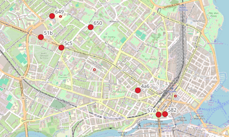
Below is a map, showing the seven sensors (red points), with their identifier deveui.

How to compute the assimilation?

To compute the data assimilation, you will have to execute several WPS .groovy scripts. You can play with them in two ways:

with the NoiseModelling’s GUI (Graphic User Interface). In this case, the WPS blocks are listed in the Data_Assimilation tab (see screenshot below),
in command line (see how to Pilot NoiseModelling with scripts). In this case, just note that they are stored in the folder .../NoiseModelling_5.0.1/data_dir/scripts/wps/DataAssimilation/,
in a .groovy script, calling one or various WPS .groovy scripts.

Data Simulation

This process prepares the training dataset from sensor measurements, importing it into NoiseModelling (in a spatial database) and performing various calculations to determine noise levels.

Maps are generated with all possible combinations, in order to identify the best road configuration in terms of noise levels generated.

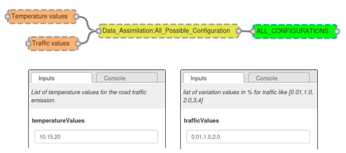
Step 1 : Generate all possible combinations

Generates all possible combinations of values from two given lists and inserts them into a table named ALL_CONFIGURATIONS.

To calculate the combinations, you have to execute the WPS script All_Possible_Configuration.

Two input parameters are needed:

Traffic values (trafficValues): variation around standard values for the 4 types of roads: primary, secondary, tertiary and others. When generating a variation of the default map (the set of maps), the values taken by the primary, the secondary, … sections, will be calculated from these parameters (between 1 and n). For example, if "trafficValues": "0.01, 1", then the primary sections will take 1% or 100% of their default value. The same applies to the remaining road types.
Temperature values (temperatureValues) : the temperatures (in °C - Double). The 1 to n possible temperatures to play (in the example below, 3 temperatures are defined: 10, 15 and 20°C)

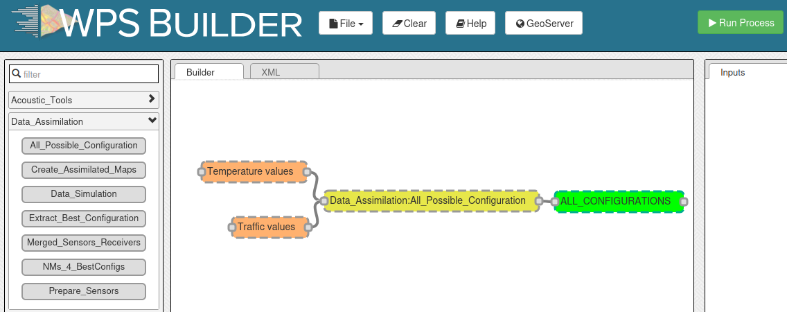
Execute `All_Possible_Configuration` WPS block

With the NoiseModelling GUI

With command lines

cd /home/.../NoiseModelling_5.0.1/

./bin/wps_scripts -w ./ -s data_dir/scripts/wps/Data_Assimilation/All_Possible_Configuration.groovy -trafficValues "0.01,1,2" -temperatureValues "10,15,20"

With Groovy script

new All_Possible_Configuration().exec(connection,[
               "trafficValues": "0.01,1.0,2.0",
               "temperatureValues": "10,15,20"
])

Result

The generated combinations include values for type of roads primary, secondary, tertiary, others, and temperature. The resulting table ALL_CONFIGURATIONS has the following columns:

IT: Unique identifier of the combination (Primary Key - Integer)
PRIMARY_VAL: percentage of primary roads traffic, given by trafficValues (Double)
SECONDARY_VAL: … of secondary roads … (Double)
TERTIARY_VAL: … of tertiary roads …(Double)
OTHERS_VAL: … of other roads …(Double)
TEMP_VAL: temperature (Double)

The first 10 lines of this table are shown below:

IT	PRIMARY_VAL	SECONDARY_VAL	TERTIARY_VAL	OTHERS_VAL	TEMP_VAL
1	0.01	0.01	0.01	0.01	10
2	0.01	0.01	0.01	0.01	15
3	0.01	0.01	0.01	0.01	20
4	1.0	0.01	0.01	0.01	10
5	1.0	0.01	0.01	0.01	15
6	1.0	0.01	0.01	0.01	20
7	1.0	1.0	0.01	0.01	10
8	1.0	1.0	0.01	0.01	15
9	1.0	1.0	0.01	0.01	20
10	1.0	1.0	1.0	0.01	10

Warning

The total number of combinations can be huge. This value is defined as: (number of trafficValues elements) ^ 4 * (number of temperatureValues elements).

In our example, we have "trafficValues": "0.01, 1.0, 2.0" and "temperatureValues": "10,15,20", so the number of combinations = 3 ^ 4 * 3 = 243 (before filtration - see ‘note‘ tab just below)

Even though this table is very important, only part of it will be used for all the maps to be simulated (see Step 5)

Note

When the combinations are calculated, a filter is applied to remove inconsistent pairs (e.g. an ‘other’ type road with much more traffic than a ‘primary‘ road).

As a result, only pairs meeting the following rule are retained: traffic on a lower type of road / traffic on a higher type of road <= 20

This rule eliminates cases where a road of a lower type would have 20 times more traffic than another of a higher type.

Step 2 : Import sensor positions

Using the Import_File WPS script*, import the location of the sensors into the NoiseModelling’s database from the .geojson file device_mapping_sf.geojson. This file will be stored in a table called SENSORS_LOCATION.

* in the data_dir/scripts/wps/Ìmport_and_Export/ folder

🌍 Since we are in the Geneva area, we are using the CH1903+ metric coordinate system (identified as EPSG:2056).

pathFile : .../device_mapping_sf.geojson
inputSRID : 2056
tableName : SENSORS_LOCATION

If you are using the Groovy script

new Import_File().exec(connection,[
                "pathFile" : workingFolder+"device_mapping_sf.geojson",
                "inputSRID" : 2056,
                "tableName": "SENSORS_LOCATION"
])

Result

Once done, you have the table SENSORS_LOCATION, presented below.

THE_GEOM	DEVEUI
POINT Z(2499748.01396418 1118023.64763599 4)	57a
POINT Z(2497926.50847343 1119715.69600241 4)	649
POINT Z(2499855.07784477 1118032.40228679 4)	582
POINT Z(2497737.00785445 1119351.14658559 4)	51b
POINT Z(2499392.11210506 1118441.15233318 4)	4a6
POINT Z(2498584.3443027 1119522.320612 4)	650
POINT Z(2498084.77671566 1119172.90847018 4)	5c5

Step 3 : Prepare sensor data

Now we can extract and prepare the sensors, for a given period. To do so, we are using the Prepare_Sensors WPS .groovy script stored in the folder .../data_dir/scripts/wps/DataAssimilation/.

This script has the following parameters:

startDate : the start timestamp to extract the dataset (in format YYYY-MM-DD HH:MM:SS)
endDate : the start timestamp to extract the dataset (in format YYYY-MM-DD HH:MM:SS)
trainingRatio : define the percentage of data to be used for training (e.g a value of 0.7 means that 70% of the data will be used for training. The remaining 30% will be used for validation) (Double)
workingFolder : folder containing the file device_mapping_sf.csv, the OSM file and the devices_data folder.
targetSRID: Target projection identifier (also called SRID) of your project (Integer)

Execution

For this tutorial, you can fill with these informations:

startDate : 2024-08-25 06:30:00
endDate : 2024-08-25 07:30:00
trainingRatio : 0.8
workingFolder : .../data_dir/data/wpsdata/dataAssimilation/ (enter the full URL e.g /home/myUserName/Documents/NoiseModelling_5.0.0/NoiseModelling_5.0.0/data_dir/data/wpsdata/dataAssimilation/)
targetSRID : 2056

If you are using the Groovy script

new Prepare_Sensors().exec(connection,[
                "startDate":"2024-08-25 06:30:00",
                "endDate": "2024-08-25 07:30:00",
                "trainingRatio": 0.8,
                "workingFolder": ".../data_dir/data/wpsdata/dataAssimilation/",
                "targetSRID": 2056
])

Result

Once executed, two tables are created:

SENSORS_MEASUREMENTS : representing all the data for this period, with sensor’s position (POINT geometry)
SENSORS_MEASUREMENTS_TRAINING : filtering SENSORS_MEASUREMENTS to keep only the training dataset. This table (described below) will be used as the RECEIVER table for the following steps.
- IDSENSOR : Unique identifier of the sensor,
- THE_GEOM : The sensor’s position (POINT geometry),
- IDRECEIVER : The receiver’s unique Id
- EPOCH : Time of measurement (Epoch format - Unix time, ex:1724567400),
- LAEQ : Equivalent continuous sound level in dB(A), calculated over a period (15 min),
- TEMP : Temperature (°C) recorded by the sensor at the time of measurement.

Step 4: Import buildings and roads

Now, using the Ìmport_OSM block, you can import buildings and road network (with predicted traffic flows) from the geneva.osm.pbf OSM file.

Execution

Path of the OSM file (pathFile): .../data_dir/data/wpsdata/dataAssimilation/geneva.osm.pbf
Target projection identifier (targetSRID): 2056
Do not import Surface acoustic absorption (ignoreGround): true
Remove tunnels from OSM data (removeTunnels): true

The other parameters are left as default

If you are using the Groovy script

new Import_OSM().exec(connection, [
                "pathFile"      : ".../data_dir/data/wpsdata/dataAssimilation/geneva.osm.pbf",
                "targetSRID"    : 2056,
                "ignoreGround"  : true,
                "removeTunnels" : true
])

Result

The tables BUILDINGS and ROADS are created.

Note

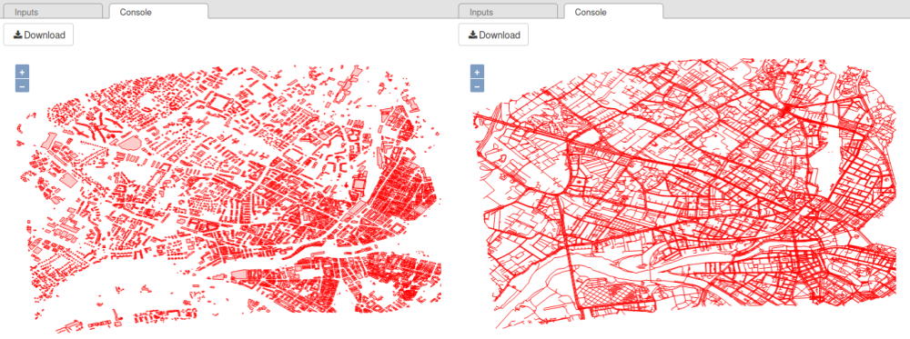
If you are using NoiseModelling with the GUI and wish to visualize the data in a map, you can use the Table_Visualization_Map block. Below is the result with the two table BUILDINGS (left) and ROADS (right).

Step 5 : Generate all traffic emissions and maps

This step consists in generating all the traffic emissions by modifying traffic data according to the road type, using data from ALL_CONFIGURATIONS (see Step 1).

1. Generate emissisons

To do so, users have first to execute the Data_Simulation WPS block, which has only one optionnal parameter :

noiseMapLimit : final number of maps to be generated (Integer). If a value is filled, a random selection is applied to keep the number of expected maps, based on the LHS (Latin Hypercube Sampling) method.

Execution

For this tutorial, you can fill with this information:

noiseMapLimit : 80

If you are using the Groovy script

new DataSimulation().exec(connection,[
                "noiseMapLimit": 80
])

Result

Two tables are created:

LW_ROADS : table containing all traffic emissions
ROADS_GEOM : table containing the geometry of roads

2. Calculate noise levels

Now, users can calculate the noise levels, emitted from the road sources. To do so, execute the Noise_level_from_source WPS script.

Execution

For this tutorial, you can fill with this information:

Source geometry table name (tableSources): ROADS_GEOM
Source emission table name (tableSourcesEmission): LW_ROADS
Buildings table name (tableBuilding): BUILDINGS
Receivers table name (tableReceivers): SENSORS_LOCATION,
Separate receiver level by source id (confExportSourceId): false
Maximum source-receiver distance (confMaxSrcDist): 250
Diffraction on vertical edges (confDiffVertical): false
Diffraction on horizontal edges (confDiffHorizontal): false

If you are using the Groovy script

new Noise_level_from_source().exec(connection, [
                "tableSources": "ROADS_GEOM",
                "tableSourcesEmission" : "LW_ROADS",
                "tableBuilding": "BUILDINGS",
                "tableReceivers": "SENSORS_LOCATION",
                "confExportSourceId": false,
                "confMaxSrcDist": 250,
                "confDiffVertical": false,
                "confDiffHorizontal": false
])

Result

The table RECEIVERS_LEVEL is created and stores all the generated maps (see the three first lines below - you can scroll the table to the right).

IDRECEIVER	PERIOD	THE_GEOM	HZ63	HZ8000	LAEQ	LEQ
1433	344	SRID=2056;POINT Z (2496912.2844730876 1116884.1525357629 4)	44.601295	14.591279	38.107693	46.40716
1433	448	SRID=2056;POINT Z (2496912.2844730876 1116884.1525357629 4)	46.617485	15.979266	40.203373	48.37574
1433	648	SRID=2056;POINT Z (2496912.2844730876 1116884.1525357629 4)	46.617485	15.979266	40.203373	48.37574

Step 6 : Extract best configuration

Many maps have been generated. So now, the best map, minimizing the difference between the measurements and the simulation, must be chosen.

To do so, users have to execute the Extract_Best_Configuration WPS script. There are 3 parameters to enter here:

Measurement table (observationTable): name of the table where observed data are stored,
Noise map table (noiseMapTable): name of the table where simulated data are stored,
Temperature tolerance threshold (tempToleranceThreshold): tolerance threshold (exprimed in °C) for the temperature that allows to extract the map that have a temperature value close to the real temperature.

This process will:

first determine the LAEQ difference between simulated (noiseMapTable) and observed (observationTable) values,
then calculate, for each time steps and for all maps, the median value of the difference between the two values. The map having the smallest median value will be the best one.

Execution

For this tutorial, you can fill with this information:

observationTable : SENSORS_MEASUREMENTS_TRAINING
noiseMapTable : RECEIVERS_LEVEL
tempToleranceThreshold : 5

If you are using the Groovy script

new Extract_Best_Configuration().exec(connection,[
                "observationTable": "SENSORS_MEASUREMENTS_TRAINING",
                "noiseMapTable": "RECEIVERS_LEVEL",
                "tempToleranceThreshold"  : 5
])

Result

Note

The best configuration is found for each time step (here 15 minutes)

As a result, the BEST_CONFIGURATION_FULL table is created (see table below). This table is made of the following columns:

EPOCH : Time of measurement (Epoch format - Unix time, ex:1724567400),
MIN_MEDIAN_DIFF : the minimum median of the difference between simulated and measured LAEQs (this is how the best maps are chosen)
IT : Unique identifier of the combination (Primary Key - Integer)
PRIMARY_VAL : percentage of primary roads traffic, given by trafficValues (Double)
SECONDARY_VAL : … secondary roads …
TERTIARY_VAL : … tertiary roads …
OTHERS_VAL : … other roads …
TEMP_VAL : temperature (Interger)

Table `BEST_CONFIGURATION_FULL` showing one best configuration for each of the time steps
EPOCH	MIN_MEDIAN_DIFF	IT	PRIMARY_VAL	SECONDARY_VAL	TERTIARY_VAL	OTHERS_VAL	TEMP_VAL
1724567400	9.3827	366	2.8	2.8	0.01	0.2	10
1724569200	11.2629	577	3.0	0.2	3.0	0.2	15
1724570100	11.2	577	3.0	0.2	3.0	0.2	15
1724571000	11.625	577	3.0	0.2	3.0	0.2	15
1724568300	11.1953	679	3.0	3.0	0.2	0.2	25
1724569201	7.8047	679	3.0	3.0	0.2	0.2	25
1724569202	10.3047	679	3.0	3.0	0.2	0.2	25

Execute Simulation: Generate the Dynamic Map

This part is made to execute a dynamic traffic calibration process, using the best configuration.

Step 7 : Generate new receivers

Create a regular grid of receivers between the buildings.

To do so, use the Regular_Grid WPS script (in the /Receivers/ wps scripts folder).

Execution

For this tutorial, you can fill with this information:

Buildings table name (buildingTableName): BUILDINGS
Table bounding box name (fenceTableName): BUILDINGS
Source table name (sourcesTableName): ROADS
Offset (delta): 200 (1 receiver every 200m)

If you are using the Groovy script

new Regular_Grid().exec(connection,[
              "buildingTableName": "BUILDINGS",
              "fenceTableName": "BUILDINGS",
              "sourcesTableName":"ROADS",
              "delta": 200
])

Result

The table RECEIVERS is created.

Three first lines of the table `RECEIVERS`
THE_GEOM	ID_COL	ID_ROW	PK
POINT Z(2496682.2844730876 1116854.1525357629 4)	1	1	1
POINT Z(2496882.2844730876 1116854.1525357629 4)	2	1	2
POINT Z(2497482.2844730876 1116854.1525357629 4)	5	1	5

Step 8 : Adding sensors as receivers

Optionally, add the sensors location into the RECEIVERS table (just created before).

Execution

In the Merged_Sensors_Receivers WPS block, fill these information:

The receiver table (tableReceivers): RECEIVERS
The sensors table (tableSensors): SENSORS_LOCATION

If you are using the Groovy script

new Merged_Sensors_Receivers().exec(connection,[
                "tableReceivers": "RECEIVERS",
                "tableSensors" : "SENSORS_LOCATION"
])

Result

The RECEIVERS table has now new points, the sensor’s one

Step 9 : Generate dynamic road emissions

For each time step (here 15 min), generate an emissions map for all the receivers, corresponding to the best configuration (for this time step).

To do so, use the NMs_4_BestConfigs WPS block. This block has two inputs:

The best configuration table (bestConfig)
The road emission table (roadEmission)

Execution

bestConfig : BEST_CONFIGURATION_FULL
roadEmission : LW_ROADS

If you are using the Groovy script

new NMs_4_BestConfigs().exec(connection)
                "bestConfig": "BEST_CONFIGURATION_FULL",
                "roadEmission" : "LW_ROADS"

Result

The table LW_ROADS_best is created, with the following structure:

PK : Unique Identifier
IDSOURCE : Source id
PERIOD : time
HZ63 : noise level for the 63 HZ frequency band
HZ125 : … for 125 HZ …
HZ250 : … for 250 HZ …
HZ500 : … for 500 HZ …
HZ1000 : … for 1000 HZ …
HZ2000 : … for 2000 HZ …
HZ4000 : … for 4000 HZ …
HZ8000 : … for 8000 HZ …

Step 10 : Generate the noise levels

Using the Noise_level_from_source WPS block, we can finally compute the noise level from the network sources emission (LW_ROADS_best) based on all the receivers.

Execution

Source geometry table name (tableSources): ROADS_GEOM
Source emission table name (tableSourcesEmission): LW_ROADS_best
Buildings table name (tableBuilding): BUILDINGS
Receivers table name (tableReceivers): RECEIVERS
Separate receiver level by source id (confExportSourceId): false
Maximum source-receiver distance (confMaxSrcDist): 250
Diffraction on vertical edges (confDiffVertical): false
Diffraction on horizontal edges (confDiffHorizontal): false

If you are using the Groovy script

new Noise_level_from_source().exec(connection, [
                      "tableSources": "ROADS_GEOM",
                      "tableSourcesEmission" : "LW_ROADS_best",
                      "tableBuilding": "BUILDINGS",
                      "tableReceivers": "RECEIVERS",
                      "confExportSourceId": false,
                      "confMaxSrcDist": 250,
                      "confDiffVertical": false,
                      "confDiffHorizontal": false
])

Result

We obtain the table RECEIVERS_LEVEL.

Step 11 : Create & visualize the resulting table

Create a table, called ASSIMILATED_MAPS, containing both sound levels and configuration parameters.

To do so, execute the Create_Assimilated_Maps WPS block, with the 3 following parameters:

bestConfigTable : the best configuration table name
receiverLevel : the receivers level table name
outputTable : the output table name

Execution

For this tutorial, you can fill with this information:

bestConfigTable : BEST_CONFIGURATION_FULL
receiverLevel : RECEIVERS_LEVEL
outputTable : ASSIMILATED_MAPS

new Create_Assimilated_Maps().exec(connection,[
                "bestConfigTable" : "BEST_CONFIGURATION_FULL",
                "receiverLevel" : "RECEIVERS_LEVEL",
                "outputTable": "ASSIMILATED_MAPS"
])

Result

The resulting ASSIMILATED_MAPS table has the following columns:

TIMESTAMP : time of the measure
LAEQ : noise level (dB(A))
THE_GEOM : receiver’s geometry (POINT)
IDRECEIVER : receiver’s unique identifier

Three first lines of the table `RECEIVERS`
TIMESTAMP	LAEQ	THE_GEOM	IDRECEIVER
1724567400	38.16436	SRID=2056;POINT Z (2496912.2844730876 1116884.1525357629 4)	1433
1724567400	39.29134	SRID=2056;POINT Z (2496912.2844730876 1116864.1525357629 4)	1197
1724567400	42.9573	SRID=2056;POINT Z (2496912.2844730876 1116844.1525357629 4)	961

Visualize the map

You can now export the ASSIMILATED_MAPS table, for example as a Shapefile, using the Export_Table WPS block and then import it into your favorite GIS app (such as QGIS) to visualize the results.

exportPath : results/ASSIMILATED_MAPS.shp
tableToExport: ASSIMILATED_MAPS

or

new Export_Table().exec(connection,
                ["exportPath": "results/ASSIMILATED_MAPS.shp",
                 "tableToExport": "ASSIMILATED_MAPS"
])

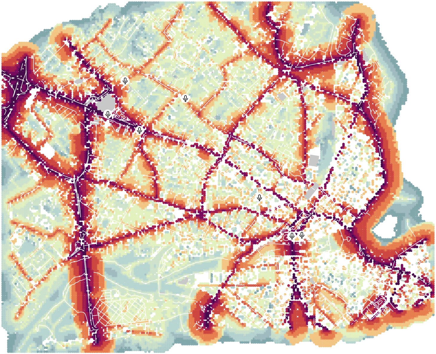
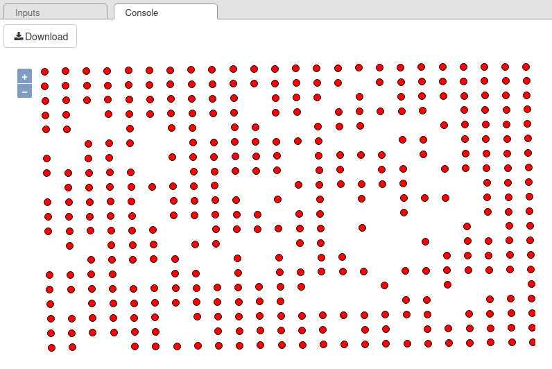
The resulting map may looks like this:

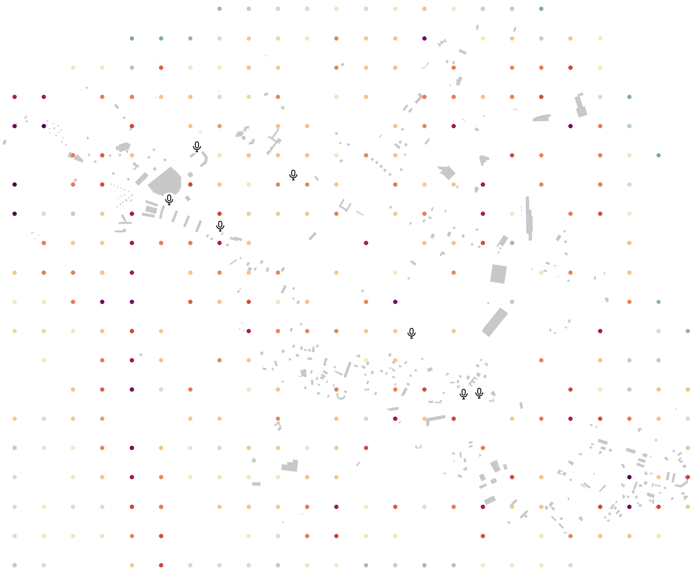
Legend: Here, we applied the color scheme proposed by Beate Tomio (see Noise Map Color Scheme) on the column LAEQ. We also added the input sensors, the buildings (light grey) and the roads (white lines).

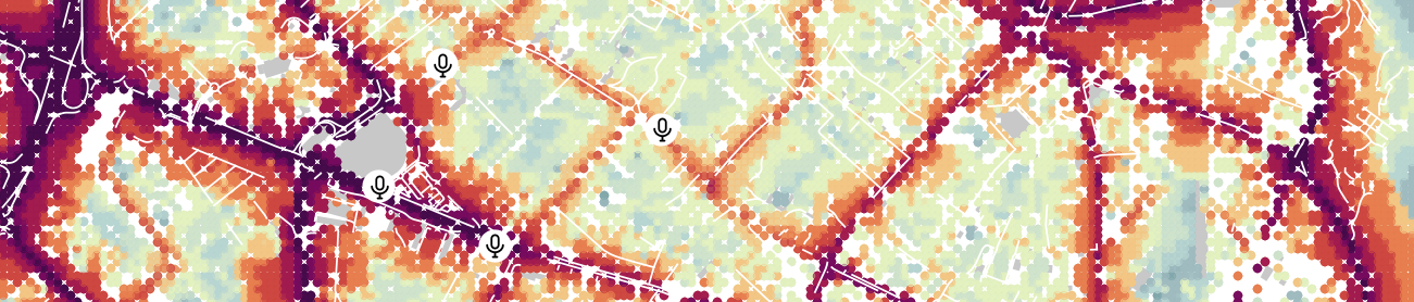
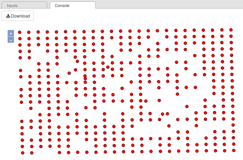
Remark: In this example, we have chosen to have a receiver every 200m (see Step 7). To achieve a denser rendering, we could have made the receiver grid denser. Below is an example, on the same area, but with a 20m grid.

Data Assimilation

Introduction

Requirements

The data

Sensor measurements

Sensor localization

How to compute the assimilation?

Data Simulation

Step 1 : Generate all possible combinations

Execute All_Possible_Configuration WPS block

Result

Step 2 : Import sensor positions

Result

Step 3 : Prepare sensor data

Execution

Result

Step 4: Import buildings and roads

Execution

Result

Step 5 : Generate all traffic emissions and maps

1. Generate emissisons

Execution

Result

2. Calculate noise levels

Execution

Result

Step 6 : Extract best configuration

Execution

Result

Execute Simulation: Generate the Dynamic Map

Step 7 : Generate new receivers

Execution

Result

Step 8 : Adding sensors as receivers

Execution

Result

Step 9 : Generate dynamic road emissions

Execution

Result

Step 10 : Generate the noise levels

Execution

Result

Step 11 : Create & visualize the resulting table

Execution

Result

Visualize the map

Execute `All_Possible_Configuration` WPS block