Get Started - GUI
Below we present a simple example to help you discover NoiseModelling through its Graphical User Interface (GUI).
Step 1: Download NoiseModelling
Download the latest release of NoiseModelling on Github.
Windows: you can directly download and run the
NoiseModelling_5.x.x_install.exeinstaller file (or you can also follow the Linux / Mac instructions below)Linux or Mac: download the
NoiseModelling_5.x.x.zipfile and unzip it into a chosen directory
Warning
The chosen directory can be anywhere, but make sure you have write access. If you are using a company computer, the Program Files folder is probably not a good idea.
Warning
For Linux and Mac users, please make sure your Java environment is correctly set up. For more information, please read the page Requirements. Windows users who are using the .exe file are not concerned, since the Java Runtime Environment is already embedded.
Note
Starting from version 3.3, NoiseModelling releases include the user interface described in this tutorial.
Step 2: Start NoiseModelling GUI
As described on the page “Architecture”, NoiseModelling can be used through a Graphical User Interface (GUI) in a web browser.
In this tutorial, we will use the default, already configured H2GIS database.
These tools (WPS Builder and H2GIS) are already included in the archive, so you don’t have to install them separately.
To launch NoiseModelling with the GUI, start it from a command prompt (terminal). This will start a local server on your computer, which provides the GUI as a web application.
Please execute:
Windows:
NoiseModelling.exeorNoiseModelling_xxx\start_windows.batLinux or Mac:
NoiseModelling_xxx/start_linux_macos.sh(make sure the file is allowed to be executed before running it)
Tip
NoiseModelling will stay open as long as the command window is open. If you close it, NoiseModelling will automatically stop and the GUI will no longer be available.
Step 3: Open NoiseModelling GUI
The NoiseModelling GUI is built using the WPS Builder component and runs as a web application provided by the local server started in Step 2.
By running NoiseModelling your default web browser should have been opened to the http://localhost:8000 address. If not please go to this URL, if something went wrong you should have more information on your terminal.
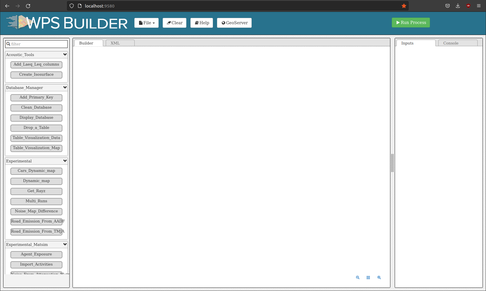
You are now ready to discover the power of NoiseModelling!
Step 4: Load input files
To compute your first noise map, you need to load input geographic files into the NoiseModelling database.
In this tutorial, we have 5 layers, zoomed in on the city center of Lorient (France): Buildings, Roads, Ground type, Topography (DEM) and Receivers.
In the resources/ sub-folder of the NoiseModelling installation, you will find all the data that will be used in the tutorials.
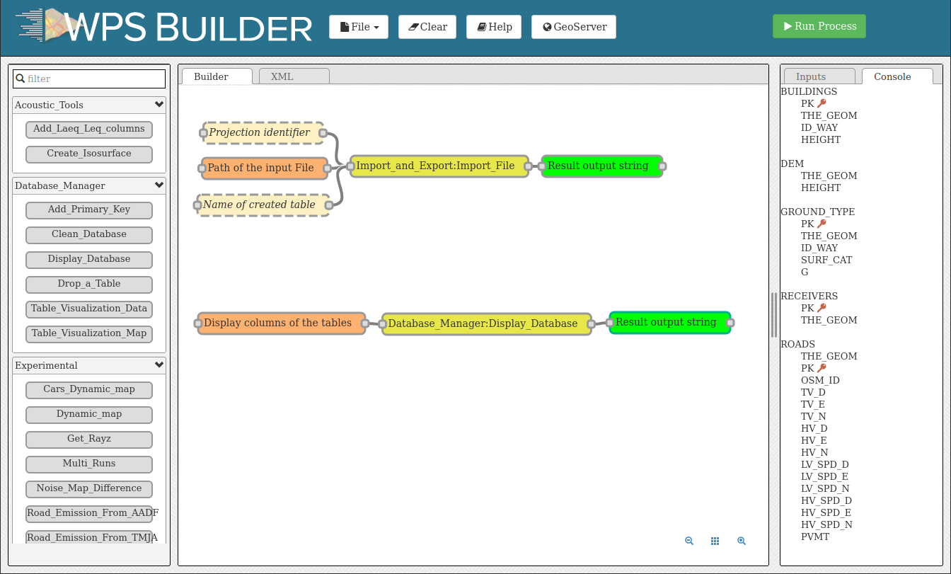
You will import these layers into your database using the Import File blocks.
Drag the
Import Fileblock into the Builder windowSelect the
Path of the input Filebox and enterresources/buildings.shpin thePathFilefield (on the right-side column)Then click on
Run Processafter selecting one of the input/output boxes of your process
Repeat this operation for the 4 other files:
resources/ground_type.shpresources/receivers.shpresources/ROADS2.shpresources/dem.geojson
Files are uploaded to the database when the Console window displays the name of the layer.
Note
If you get the message
Error opening database, please refer to the note in Step 1.The process is supposed to be quick (<5 sec.). In case of a timeout, try restarting NoiseModelling (see Step 2).
Orange blocks are mandatory
Beige blocks are optional
If all input blocks are optional, you must modify at least one of these blocks to be able to run the process
Blocks get a solid border when they are ready to run
Read the WPS Builder page for more information
Once done, you can check whether the tables were correctly imported into the database. To do so, drag/drop and execute the Display_Database WPS script (in the “Database_Manager” part). You should see on the right panel the table list (and their columns if you checked the option in the Display columns of the tables block).
Step 5: Run Calculation
To run the calculation, drag the Noise_level_from_traffic block into the WPS Builder window.
Then, select the orange blocks and enter the name of the corresponding table in your database:
Building table name:
BUILDINGSSources table name:
ROADS2This table contains the road geometries with traffic data for day, evening and nightReceivers table name:
RECEIVERSLocations where noise levels are evaluatedDEM table name:
DEMDigital elevation modelGround absorption table:
GROUND_TYPENature of the groundDiffraction on horizontal edges:
☑check it (sound propagation goes over buildings)Maximum source-receiver distance: set
2000meters (do not look for sound sources further than 2 km)Order of reflection: set
0to disable it (faster but less accurate)
The beige blocks correspond to optional parameters (e.g. DEM table name, Ground absorption table name, Diffraction on vertical edges, …).
When ready, you can press Run Process.
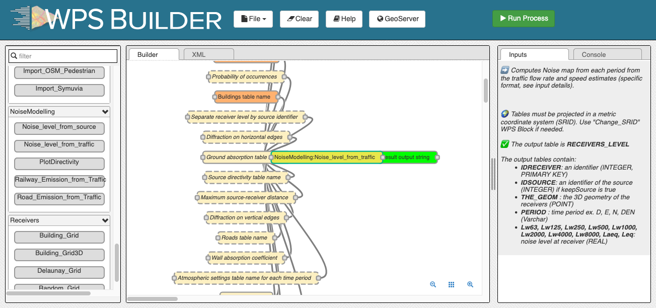
As a result, the table RECEIVERS_LEVEL will be created in your database. This table corresponds to the noise levels computed at receiver points. The column PERIOD corresponds to the 4 different periods of the day (D, E, N and DEN).
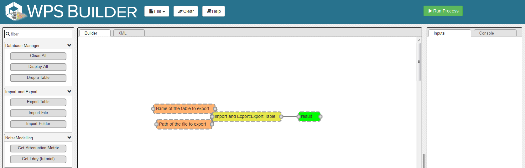
Step 6: Export (& see) the results
You can now export the output tables (one by one) in your preferred export format using the Export_Table block, giving the path of the file you want to create.
Warning
Don’t forget to add the file extension (e.g. c:/home/receivers_level.geojson or c:/home/receivers_level.shp). (Read more info about file extensions here: Tutorials - FAQ)
For example, you can export the tables in .shp format. This format can be read with most GIS tools such as the free and open-source QGIS and SAGA software.
Note
For those who are new to GIS and want to get started with QGIS, we advise you to follow this tutorial.
To obtain the following image, use the styling options in your GIS and assign a color gradient to the LAEQ column of your exported RECEIVERS_LEVEL table.
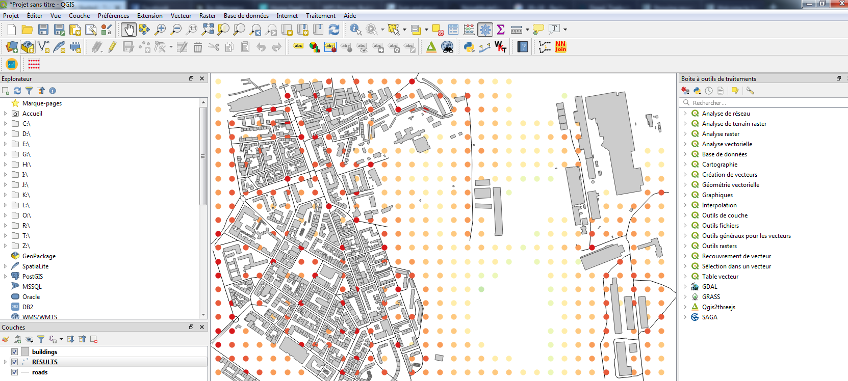
To display the result for a specific period, filter the rendering by the field PERIOD in QGIS.
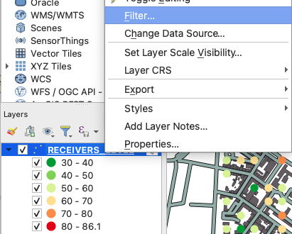
Popup menu
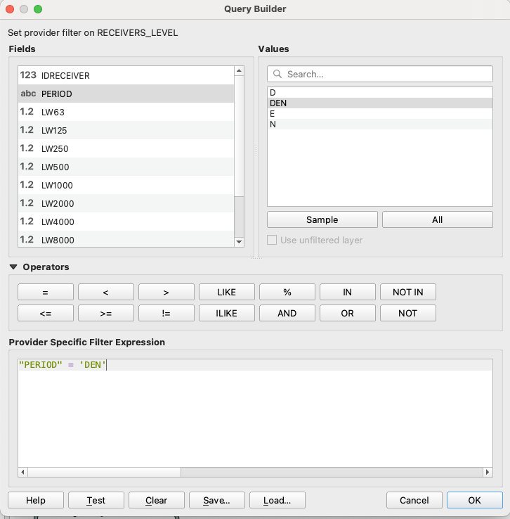
Filter window
Tip
Now that you have made your first noise map (congratulations!), you can try again by adding or changing optional parameters to see the differences.
Step 7: Know the possibilities
Now that you have finished this introduction tutorial, take the time to read the description of each of the WPS blocks available in your NoiseModelling version.
By clicking on each of the inputs or outputs, you will find a lot of information.