Vibration of a beam clamped at one end

The beam is increasingly loaded at its other end, and then suddenly released.

• Time-domain, implicit scheme

• 3D

• Rayleigh damping

This example is adapted from (legacy Fenics):

  https://comet-fenics.readthedocs.io/en/latest/demo/elastodynamics/demo_elastodynamics.py.html

where extensive explanations are given. Here we show how elastodynamicsx can be used to reproduce it.

import numpy as np

from dolfinx import mesh, fem, default_scalar_type
from mpi4py import MPI

from elastodynamicsx.pde import material, boundarycondition, PDE, damping
from elastodynamicsx.solvers import TimeStepper
from elastodynamicsx.utils import make_facet_tags, ParallelEvaluator

FE domain

L_, B_, H_ = 1, 0.04, 0.1
Nx, Ny, Nz = 60, 5, 10  # Nb of elts.

extent = [[0., 0., 0.], [L_, B_, H_]]

# create the mesh
domain = mesh.create_box(MPI.COMM_WORLD, extent, [Nx, Ny, Nz])

# create the function space
V = fem.functionspace(domain, ("Lagrange", 1, (domain.geometry.dim,)))

# define some tags
tag_left, tag_top, tag_right, tag_bottom, tag_back, tag_front = 1, 2, 3, 4, 5, 6
boundaries = [(tag_left  , lambda x: np.isclose(x[0], 0.)),
              (tag_right , lambda x: np.isclose(x[0], L_)),
              (tag_bottom, lambda x: np.isclose(x[1], 0.)),
              (tag_top   , lambda x: np.isclose(x[1], B_)),
              (tag_back  , lambda x: np.isclose(x[2], 0.)),
              (tag_front , lambda x: np.isclose(x[2], H_))]

facet_tags = make_facet_tags(domain, boundaries)

Boundary conditions

• Clamp the left face

• Apply a load on the right face

# Left: clamp
bc_l = boundarycondition((V, facet_tags, tag_left), 'Clamp')

# Right: normal traction (Neumann boundary condition)
T_N  = fem.Constant(domain, np.array([0] * 3, dtype=default_scalar_type))
bc_r = boundarycondition((V, facet_tags, tag_right), 'Neumann', T_N)

bcs  = [bc_l, bc_r]  # list all BCs

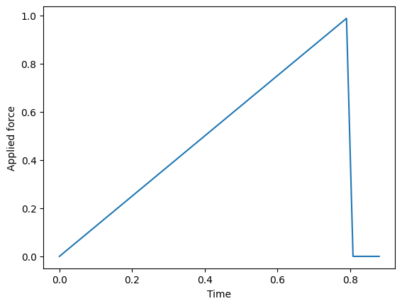
Define the temporal behavior of the source

# -> Time function
p_0 = 1.  # max amplitude
F_0 = p_0 * np.array([0, 0, 1], dtype=default_scalar_type)  # source orientation
cutoff_Tc = 4 / 5  # release time

src_t        = lambda t: t / cutoff_Tc * (t > 0) * (t <= cutoff_Tc)
T_N_function = lambda t: src_t(t) * F_0

if domain.comm.rank == 0:
    import matplotlib.pyplot as plt
    t = np.linspace(0, 1.1 * cutoff_Tc)
    plt.plot(t, src_t(t))
    plt.xlabel('Time')
    plt.ylabel('Applied force')
    plt.show()

Define the material law

• isotropic elasticity

• with Rayleigh damping: \([C] = \eta_M [M] + \eta_K [K]\) where \([M]\), \([K]\) and \([C]\) are the mass, stiffness and damping matrices

# Parameters here...
E, nu = 1000, 0.3  # Young's modulus and Poisson's ratio
rho = 1  # mass density

eta_m = 0.01  # Rayleigh damping param
eta_k = 0.01  # Rayleigh damping param
# ... end

# Convert Young & Poisson to Lamé's constants
lambda_ = E * nu / (1 + nu) / (1 - 2 * nu)
mu      = E / 2 / (1 + nu)

# Convert floats to fem.Constant
rho     = fem.Constant(domain, default_scalar_type(rho))
lambda_ = fem.Constant(domain, default_scalar_type(lambda_))
mu      = fem.Constant(domain, default_scalar_type(mu))
eta_m = fem.Constant(domain, default_scalar_type(eta_m))
eta_k = fem.Constant(domain, default_scalar_type(eta_k))

material = material(V,
                    'isotropic',
                    rho, lambda_, mu,
                    damping=damping('Rayleigh', eta_m, eta_k))

Assemble the PDE

pde = PDE(V, materials=[material], bodyforces=[], bcs=bcs)

Time scheme

We use the Generalized-alpha method, which is an explicit scheme that can be viewed as an extention of the Newmark-\(\beta\) family. The parameters of the scheme are \(\alpha_m\), \(\alpha_f\), \(\gamma\), \(\beta\). Here we take: - \(\alpha_m=0.2\), - \(\alpha_f=0.4\),

while the other parameters are set by default to \(\gamma=\frac{1}{2} + \alpha_f - \alpha_m\) and \(\beta = \frac{1}{4}(\gamma + \frac{1}{2})^2\) to ensure second order accuracy, and stability. Note that stability is only unconditionnal in the linear, non dissipative case.

See:

 J. Chung and G. M. Hulbert, A time integration algorithm for structural dynamics with improved numerical dissipation: The generalized-α method,J. Appl. Mech. 60(2), 371–375 (1993).

# Temporal parameters
T      = 4  # duration; difference with original example: here t=[0,T-dt]
Nsteps = 50  # number of time steps
dt = T / Nsteps  # time increment

# Generalized-alpha method parameters
alpha_m = 0.2
alpha_f = 0.4
kwargsTScheme = dict(scheme='g-a-newmark', alpha_m=alpha_m, alpha_f=alpha_f)

# Time integration: define a TimeStepper instance
tStepper = TimeStepper.build(V,
                             pde.M_fn, pde.C_fn, pde.K_fn, pde.b_fn, dt, bcs=bcs,
                             **kwargsTScheme)

# Set the initial values
tStepper.set_initial_condition(u0=[0, 0, 0], v0=[0, 0, 0], t0=0)

Define outputs

• Extract signals at few points

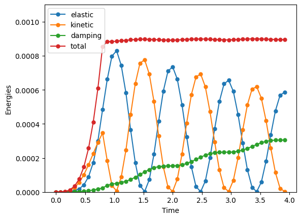
• Compute the kinetic, elastic and damping energies

• Live-plot results (only in a terminal; not in a notebook)

# -> Point evaluation
# Define points
points_out = np.array([[L_, B_ / 2, 0]]).T

# Declare a convenience ParallelEvaluator
paraEval = ParallelEvaluator(domain, points_out)

# Declare data (local process)
signals_local = np.zeros((paraEval.nb_points_local,
                          V.num_sub_spaces,
                          Nsteps))  # <- output stored here

# -> Energies
energies = np.zeros((Nsteps, 4))
E_damp = 0  # declare; init value

u_n = tStepper.timescheme.u  # The displacement at time t_n
v_n = tStepper.timescheme.v  # The velocity at time t_n
comm = V.mesh.comm


def Energy_elastic():
    return comm.allreduce(fem.assemble_scalar(fem.form(1/2 * pde.K_fn(u_n, u_n))), op=MPI.SUM)


def Energy_kinetic():
    return comm.allreduce(fem.assemble_scalar(fem.form(1/2 * pde.M_fn(v_n, v_n))), op=MPI.SUM)


def Energy_damping():
    return dt * comm.allreduce(fem.assemble_scalar(fem.form(pde.C_fn(v_n, v_n))), op=MPI.SUM)


# -> live plotting parameters
clim = 0.4 * L_ * B_ * H_ / (E * B_ * H_**3 / 12) * np.amax(F_0) * np.array([0, 1])
live_plotter = {'refresh_step': 1, 'clim': clim, 'window_size': [640, 480]} if domain.comm.rank == 0 else None


# -> Define callbacks: will be called at the end of each iteration
def cbck_storeAtPoints(i, out):
    if paraEval.nb_points_local > 0:
        signals_local[:, :, i+1] = u_n.eval(paraEval.points_local, paraEval.cells_local)


def cbck_energies(i, out):
    global E_damp
    E_elas = Energy_elastic()
    E_kin  = Energy_kinetic()
    E_damp+= Energy_damping()
    E_tot  = E_elas + E_kin + E_damp
    energies[i+1, :] = np.array([E_elas, E_kin, E_damp, E_tot])

Solve

• Define a ‘callfirst’ function to update the load BC

• Run the time loop

# 'callfirsts': will be called at the beginning of each iteration
def cfst_updateSources(t):
    T_N.value = T_N_function(t)


# Run the big time loop!
tStepper.solve(Nsteps - 1,
               callfirsts=[cfst_updateSources],
               callbacks=[cbck_storeAtPoints, cbck_energies],
               live_plotter=live_plotter)
# End of big calc.

Post-processing

Plot tip displacement and energies evolution

# Gather the data to the root process
all_signals = paraEval.gather(signals_local, root=0)

# Plot only on rank == 0
if domain.comm.rank == 0:
    t = dt * np.arange(energies.shape[0])

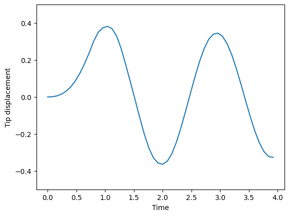
    # Tip displacement
    u_tip = all_signals[0]
    plt.figure()
    plt.plot(t, u_tip[2, :])
    plt.xlabel('Time')
    plt.ylabel('Tip displacement')
    plt.ylim(-0.5, 0.5)

    # Energies
    plt.figure()
    plt.plot(t, energies, marker='o', ms=5)
    plt.legend(("elastic", "kinetic", "damping", "total"))
    plt.xlabel("Time")
    plt.ylabel("Energies")
    plt.ylim(0, 0.0011)
    plt.show()