Self-interaction of a P wave in a 1D nonlinear elastic medium
Time-domain, explicit scheme, Spectral elements
1D
Murnaghan hyperelasticity
P-wave harmonics generation
[1]:
import numpy as np

from dolfinx import mesh, fem, default_scalar_type
import ufl
from mpi4py import MPI
from petsc4py import PETSc

from elastodynamicsx.pde import material, boundarycondition, PDE, PDECONFIG
from elastodynamicsx.solvers import TimeStepper
from elastodynamicsx.plot import plotter
from elastodynamicsx.utils import spectral_element, spectral_quadrature, make_facet_tags, ParallelEvaluator
Set up a Spectral Element Method
[2]:
degElement, nameElement = 4, "GLL"
PDECONFIG.default_metadata = spectral_quadrature(nameElement, degElement)

cell_type = mesh.CellType.interval
specFE = spectral_element(nameElement, cell_type, degElement, (2,))
FE domain
[3]:
length = 10
Nx     = 100 // degElement  # Nb of elts

# create the mesh
extent = [0, length]
domain = mesh.create_interval(MPI.COMM_WORLD, Nx, extent)

# create the function space
V = fem.functionspace(domain, specFE)

# define some tags
tag_left, tag_right = 1, 2
all_tags = (tag_left, tag_right)
boundaries = [(tag_left , lambda x: np.isclose(x[0], 0     )),
              (tag_right, lambda x: np.isclose(x[0], length))]

facet_tags = make_facet_tags(domain, boundaries)
Define the material law
Murnaghan’s hyperelasticity. Parameters:
\(\rho\): density
\(\lambda\), \(\mu\): Lamé’s constants
\(l\), \(m\), \(n\): Murnaghan’s constants
[4]:
# parameters here...
rho     = fem.Constant(domain, default_scalar_type(1))
mu      = fem.Constant(domain, default_scalar_type(1))
lambda_ = fem.Constant(domain, default_scalar_type(2))
l_      = fem.Constant(domain, default_scalar_type(1))
m_      = fem.Constant(domain, default_scalar_type(1))
n_      = fem.Constant(domain, default_scalar_type(1))
# ... end

mat = material(V, 'murnaghan', rho, lambda_, mu, l_, m_, n_)
Boundary conditions
Impedance boundary condition on either edge
Traction load \(T_N\) on the left edge, with compressive \(_x\) and shear \(_y\) components
[5]:
T_N = fem.Constant(domain, default_scalar_type([0, 0]))  # normal traction (Neumann boundary condition)
Z_N, Z_T = mat.Z_N, mat.Z_T  # P and S mechanical impedances
bc_l  = boundarycondition((V, facet_tags, tag_left), 'Neumann', T_N)
bc_rl = boundarycondition((V, facet_tags, (tag_left, tag_right)), 'Dashpot', Z_N, Z_T)

bcs = [bc_l, bc_rl]
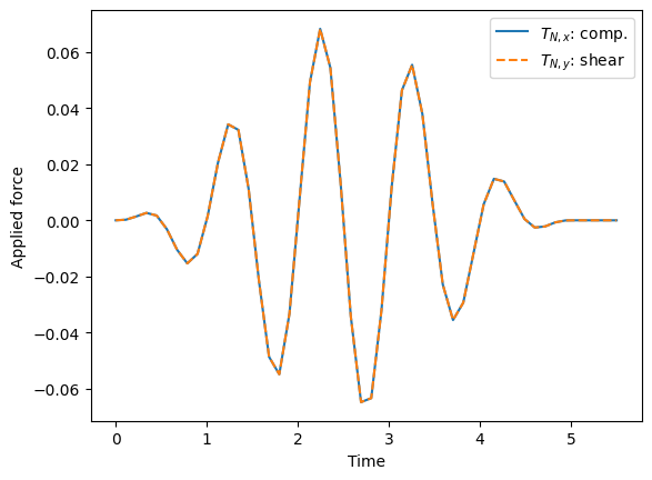
Define the temporal behavior of the source
[6]:
# -> Time function
f0 = 1       # central frequency of the source
T0 = 1 / f0  # period
d0 = 5 * T0  # duration of source


def src_t(t):  # source(t): Sine x Hann window
    window = np.sin(np.pi * t / d0)**2 * (t < d0) * (t > 0)  # Hann window
    return np.sin(2 * np.pi * f0 * t) * window


# -> Space-Time function
p_0 = default_scalar_type(7e-2)  # max amplitude
F_0 = p_0 * default_scalar_type([1, 1])  # source orientation


def T_N_function(t):
    return src_t(t) * F_0


if domain.comm.rank == 0:
    import matplotlib.pyplot as plt
    t = np.linspace(0, 1.1 * d0)
    plt.plot(t, src_t(t) * F_0[0], label=r'$T_{N,x}$: comp.')
    plt.plot(t, src_t(t) * F_0[1], ls='--', label=r'$T_{N,y}$: shear')
    plt.legend()
    plt.xlabel('Time')
    plt.ylabel('Applied force')
    plt.show()
Assemble the PDE
[7]:
pde = PDE(V, materials=[mat], bodyforces=[], bcs=bcs)
Time scheme
Leapfrog
[8]:
# Temporal parameters
tstart = 0  # Start time
tmax   = 15 * T0  # Final time
num_steps = 1500
dt = (tmax - tstart) / num_steps  # time step size

# Some control numbers...
hx = length / Nx
c_S = np.sqrt(mu.value / rho.value)  # S-wave velocity
lbda0 = c_S / f0
courant_number = TimeStepper.Courant_number(V.mesh, ufl.sqrt((lambda_ + 2 * mu) / rho), dt)
PETSc.Sys.Print(f'Number of points per wavelength at central frequency: {lbda0 / hx:.2f}')
PETSc.Sys.Print(f'Number of time steps per period at central frequency: {T0 / dt:.2f}')
PETSc.Sys.Print(f'CFL condition: Courant number = {courant_number:.2f}')

# Time integration
#     diagonal=True assumes the left hand side operator is indeed diagonal
tStepper = TimeStepper.build(V,
                             pde.M_fn, pde.C_fn, pde.K_fn, pde.b_fn, dt, bcs=bcs,
                             scheme='leapfrog', diagonal=True)

# Set the initial values
tStepper.set_initial_condition(u0=[0, 0], v0=[0, 0], t0=tstart)
Number of points per wavelength at central frequency: 2.50
Number of time steps per period at central frequency: 100.00
CFL condition: Courant number = 0.05
Define outputs
Extract signals at few points
Live-plot results (only in a terminal; not in a notebook)
[9]:
u_res = tStepper.timescheme.u  # The solution

# -> Extract signals at few points
# Define points
points_out = np.array([[3, 0, 0], [6, 0, 0], [9, 0, 0]]).T  # shape = (3, nbpts)

# Declare a convenience ParallelEvaluator
paraEval = ParallelEvaluator(domain, points_out)

# Declare data (local)
signals_local = np.zeros((paraEval.nb_points_local,
                          V.num_sub_spaces,
                          num_steps))  # <- output stored here


# -> Define callbacks: will be called at the end of each iteration
def cbck_storeAtPoints(i, out):
    if paraEval.nb_points_local > 0:
        signals_local[:, :, i+1] = u_res.eval(paraEval.points_local, paraEval.cells_local)


# enable live plotting
enable_plot = True
clim = 0.1 * np.amax(F_0) * np.array([0, 1])
kwplot = {'clim': clim, 'warp_factor': 0.5 / np.amax(clim)}
if domain.comm.rank == 0 and enable_plot:
    p = plotter(u_res, refresh_step=10, window_size=[640, 480], **kwplot)
    if paraEval.nb_points_local > 0:
        # add points to live_plotter
        p.add_points(paraEval.points_local, render_points_as_spheres=True, point_size=12)
else:
    p = None
Solve
Define a ‘callfirst’ function to update the load
Run the time loop
[10]:
# 'callfirsts': will be called at the beginning of each iteration
def cfst_updateSources(t):
    T_N.value = T_N_function(t)


# Run the big time loop!
tStepper.solve(num_steps - 1,
               callfirsts=[cfst_updateSources],
               callbacks=[cbck_storeAtPoints],
               live_plotter=p)
# End of big calc.
Post-processing
Plot signals at few points
[11]:
# Gather the data to the root process
all_signals = paraEval.gather(signals_local, root=0)
if domain.comm.rank == 0:
# -> Exact (linear) solution, At few points
x = points_out.T
t = dt * np.arange(num_steps)
cL = np.sqrt((lambda_.value + 2 * mu.value) / rho.value)
cS = np.sqrt(mu.value / rho.value)
resp_L = np.cumsum(src_t(t[np.newaxis, :] - x[:, 0, np.newaxis] / cL) * F_0[0] / 2 / cL / rho.value, axis=1) * dt
resp_S = np.cumsum(src_t(t[np.newaxis, :] - x[:, 0, np.newaxis] / cS) * F_0[1] / 2 / cS / rho.value, axis=1) * dt
signals_linear = np.stack((resp_L, resp_S), axis=1)
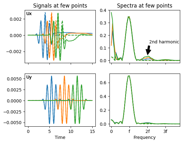
f = np.fft.rfftfreq(t.size) / dt
fig, ax = plt.subplots(V.num_sub_spaces, 2, sharex='col', sharey='none')
ax[0, 0].set_title('Signals at few points')
ax[0, 1].set_title('Spectra at few points')
for icomp, cax in enumerate(ax):
for i in range(len(all_signals)):
cax[0].text(0.02, 0.97, 'U' + ['x', 'y', 'z'][icomp], ha='left', va='top', transform=cax[0].transAxes)
cax[0].plot(t, all_signals[i, icomp, :], c=f'C{i}', ls='-') # FEM
cax[0].plot(t, signals_linear[i, icomp, :], c=f'C{i}', ls='--') # exact linear
#
cax[1].plot(f, np.abs(np.fft.rfft(all_signals[i, icomp, :])), c=f'C{i}', ls='-') # FEM
cax[1].plot(f, np.abs(np.fft.rfft(signals_linear[i, icomp, :])), c=f'C{i}', ls='--') # exact linear
specX = np.abs(np.fft.rfft(all_signals[i, 0, :]))
specX_f = specX[np.argmin(np.abs(f - 1 / T0))]
specX_2f = specX[np.argmin(np.abs(f - 2 / T0))]
ax[0, 1].annotate('2nd harmonic', xy=(2 / T0, 1.2 * specX_2f),
xytext=(2.1 / T0, 0.4 * specX_f),
arrowprops=dict(facecolor='black', shrink=0.05))
ax[-1, 0].set_xlabel('Time')
ax[-1, 1].set_xlabel('Frequency')
ax[-1, 1].set_xlim(-0.1 / T0, 3.8 / T0)
ax[-1, 1].set_xticks(np.arange(4) / T0, ['0', 'f', '2f', '3f'])
plt.show()
#
# -----------------------------------------------------